Characterization of Discrete Systems in the Spectral Domain
This Jupyter notebook is part of a collection of notebooks in the bachelors module Signals and Systems, Communications Engineering, Universität Rostock. Please direct questions and suggestions to Sascha.Spors@uni-rostock.de.
Magnitude and Phase
The discrete-time Fourier domain transfer function $H(e^{j \Omega})$ characterizes the transmission properties of a linear time-invariant (LTI) system with respect to an harmonic exponential signal $e^{j \Omega k}$ with normalized frequency $\Omega$. In order to investigate the characteristics of an LTI system, often the magnitude $| H(e^{j \Omega}) |$ and phase $\varphi_H(e^{j \Omega})$ of the transfer function are regarded separately. Decomposing the output signal $Y(e^{j \Omega}) = X(e^{j \Omega}) \cdot H(e^{j \Omega})$ into its magnitude $| Y(e^{j \Omega}) |$ and phase $\varphi_Y(e^{j \Omega})$ yields
\begin{align} | Y(e^{j \Omega}) | &= | X(e^{j \Omega}) | \cdot | H(e^{j \Omega}) | \\ \varphi_Y(e^{j \Omega}) &= \varphi_X(e^{j \Omega}) + \varphi_H(e^{j \Omega}) \end{align}where $X(e^{j \Omega})$ denotes the input signal, and $| X(e^{j \Omega}) |$ and $\varphi_X(e^{j \Omega})$ its magnitude and phase, respectively. It can be concluded, that the magnitude $| H(e^{j \Omega}) |$ quantifies the frequency-dependent attenuation of the magnitude $| X(e^{j \Omega}) |$ of the input signal by the system, while $\varphi_H(e^{j \Omega})$ quantifies the introduced phase-shift.
A rational transfer function $H(z)$ which is composed from polynomials in $z^{-1}$ can be expressed in terms of its poles and zeros. Applying this representation to the transfer function $H(e^{j \Omega})$ in the discrete-time Fourier domain yields
\begin{equation} H(e^{j \Omega}) = K \cdot \frac{\prod_{\mu=0}^{Q} (e^{j \Omega} - z_{0 \mu})}{\prod_{\nu=0}^{P} (e^{j \Omega} - z_{\infty \nu})} \end{equation}where $z_{0 \mu}$ and $z_{\infty \nu}$ denote the $\mu$-th zero and $\nu$-th pole of $H(z)$, and $Q$ and $P$ the total number of zeros and poles, respectively. Often the logarithmic magnitude of the transfer function $20 \log_{10} | H(e^{j \Omega}) |$ in decibels (dB) is considered. The representation of amplitudes in dB is beneficial due to its clear coverage of wide amplitude ranges and convenient calculus for scaled amplitudes. Using the representation of the transfer function with respect to its poles and zeros yields for the logarithm of the magnitude and the phase
\begin{align} \log_{10} | H(e^{j \Omega}) | &= \sum_{\mu=0}^{Q} \log_{10} |e^{j \Omega} - z_{0 \mu}| - \sum_{\nu=0}^{P} \log_{10} |e^{j \Omega} - z_{\infty \nu}| + \log_{10} |K| \\ \varphi_H(e^{j \Omega}) &= \sum_{\mu=0}^{Q} \arg (e^{j \Omega} - z_{0 \mu}) - \sum_{\nu=0}^{P} \arg (e^{j \Omega} - z_{\infty \nu}) \end{align}where $\arg(\cdot)$ denotes the argument (phase) of a complex function. It can be concluded, that the individual contributions of the poles and zeros to the logarithm of the magnitude and phase can be superimposed. This fact may be exploited to estimate the frequency and phase response of discrete-time systems by considering the influence of individual poles and zeros. This is discussed in the following for a system composed from one pole and one zero ($P=Q=0$).
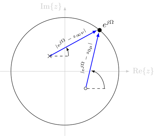
The magnitude of the transfer function depends on the ratio of Euclidean distances from the pole and zero to the position $e^{j \Omega}$ on the unit circle $|z| = 1$. Small distances, e.g. a pole or zero close to the unit circle, lead to large negative values of the individual summands in the logarithmic magnitude response, e.g. $\log_{10} |e^{j \Omega} - z_{0 \mu}|$. This holds especially for normalized frequencies $\Omega$ in the proximity of the pole/zero. It can be concluded that
- a pole close to the unit circle results in a resonance (e.g. maximum), and
- a zero close to the unit circle results in a notch/anti-resonance (e.g. minimum)
in the magnitude response. The normalized frequency $\Omega$ of this maximum/minimum is given by the argument of the pole $\arg \{ z_{\infty \mu} \}$ and zero $\arg\{ z_{0 \mu} \}$, respectively.
Example - Second order system
The magnitude response of a real-valued second-order LTI system with the specific transfer function
\begin{equation} H(e^{j \Omega}) = \frac{(e^{j \Omega} - z_0)(e^{j \Omega} - z_0^*)}{(e^{j \Omega} - z_\infty)(e^{j \Omega} - z_\infty^*)} \end{equation}is considered. It is convenient to represent the pole/zero by its magnitude and phase in order to illustrate its location relative to the unit circle
\begin{align} z_0 &= r_0 e^{j \Omega_0} &\text{with } \quad &r_0 = 0.8 & \Omega_0 = \frac{\pi}{2} \\ z_\infty &= r_\infty e^{j \Omega_\infty} & &r_\infty = 0.95 & \Omega_\infty = \frac{\pi}{4} \end{align}where for instance $r_0 = |z_0|$ and $\Omega_0 = \arg \{ z_0 \}$. First the contribution of the pair of complex conjugate zeros $z_0$ and $z_0^*$ to the logarithmic magnitude of the transfer function $H(e^{j \Omega})$ is computed and plotted over the normalized frequency $\Omega$.
import sympy as sym
%matplotlib inline
sym.init_printing()


def db(x):
    'compute dB value'
    return 20 * sym.log(sym.Abs(x), 10)


W = sym.symbols('Omega', real=True)
z_0 = 0.8 * sym.exp(sym.I * sym.pi/2)

H1 = (sym.exp(sym.I * W) - z_0)*(sym.exp(sym.I * W) - sym.conjugate(z_0))
Hlog1 = db(H1)
sym.plot(Hlog1, (W, 0, sym.pi), xlabel='$\Omega$',
         ylabel='$|H_0(e^{j \Omega})|$ in dB')
<sympy.plotting.plot.Plot at 0x118e48ba8>
Now the contribution of the pair of complex conjugate poles $z_\infty$ and $z_\infty^*$ is computed and plotted
z_inf = 0.95 * sym.exp(sym.I * sym.pi/4)

H2 = 1/((sym.exp(sym.I * W) - z_inf)*(sym.exp(sym.I * W) - sym.conjugate(z_inf)))
Hlog2 = db(H2)
sym.plot(Hlog2, (W, 0, sym.pi), xlabel='$\Omega$',
         ylabel='$|H_\infty(e^{j \Omega})|$ in dB')
<sympy.plotting.plot.Plot at 0x1193a1ef0>
The logarithmic magnitude response of the system is given by superposition of the individual contributions from the zeros and the poles
Hlog = Hlog1 + Hlog2
sym.plot(Hlog, (W, 0, sym.pi), xlabel='$\Omega$',
         ylabel='$|H(e^{j \Omega})|$ in dB')
<sympy.plotting.plot.Plot at 0x1194a4d68>
Exercise
- Why is the system real valued?
- Examine the magnitude response of the system. How is it related to the magnitude responses of the individual zeros/poles?
- Move the poles and/or zeros closer to the unit circle by changing the values $r_\infty$ and/or $r_0$. What influence does this have on the magnitude response?
- Change the phase of the pole and/or zero by changing the values $\Omega_\infty$ and/or $\Omega_0$. What influence does this have on the magnitude response?
Copyright
This notebook is provided as Open Educational Resource. Feel free to use the notebook for your own purposes. The text is licensed under Creative Commons Attribution 4.0, the code of the IPython examples under the MIT license. Please attribute the work as follows: Sascha Spors, Continuous- and Discrete-Time Signals and Systems - Theory and Computational Examples.