Shenfun - High-Performance Computing platform for the Spectral Galerkin method¶

Professor Mikael Mortensen

Department of Mathematics, University of Oslo

Presented at the International Conference on Scientific Computing and Applications (ICSCA), Xiamen, China, 29/5 - 2019

Shenfun - facts¶

1. Shenfun is named in honour of Professor Jie Shen for his seminal work on the spectral Galerkin method:-)
2. Shenfun is a high performance computing platform for solving partial differential equations (PDEs) with the spectral Galerkin method (with numerical integration).
3. Shenfun has been run with 65,000 processors on a Cray XC40.
4. Shenfun is a high-level Python package originally developed for large-scale pseudo-spectral turbulence simulations.

Python is a scripting language¶

No compilation - just execute. Much like MATLAB. High-level coding very popular in the scientific computing community.

In this presentation this is a Python terminal:

Inside the terminal any Python code can be executed and if something is printed it is shown below.

When in presentation mode¶

like now, the terminal is not alive. However, this presentation is written with jupyter

and if opened in active mode, then all boxes like the one below would be live and active and ready to execute any Python code:

If interested (it is really not necessary), then

Open https://github.com/spectralDNS/shenfun/ and press the launch-binder button.

Wait for binder to launch and choose the Shenfun presentation.ipynb file to get a live document. There are also some other demos there written in jupyter.

Meanwhile (may take a few minutes and really not necessary) I'll go through some background material required for understanding how shenfun works 😀

The Spectral Galerkin method (in a nutshell)¶

approximates solutions $u(x)$ using global trial functions $\phi_k(x)$ and unknown expansion coefficients $\hat{u}_k$

$$ u(x) = \sum_{k=0}^{N-1}\hat{u}_k \phi_k(x) $$

Multidimensional solutions are formed from outer products of 1D bases

$$ u(x, y) = \sum_{k=0}^{N_0-1}\sum_{l=0}^{N_1-1}\hat{u}_{kl} \phi_{kl}(x, y)\quad \text{ or }\quad u(x, y, z) = \sum_{k=0}^{N_0-1}\sum_{l=0}^{N_1-1} \sum_{m=0}^{N_2-1}\hat{u}_{klm} \phi_{klm}(x, y, z) $$

where, for example

$$ \begin{align} \phi_{kl}(x, y) &= T_k(x) L_l(y)\\ \phi_{klm}(x, y, z) &= T_k(x) L_l(y) \exp(\text{i}mz) \end{align} $$

$T_k$ and $L_k$ are Chebyshev and Legendre polynomials.

The Spectral Galerkin method¶

solves PDEs, like Poisson's equation

\begin{align} \nabla^2 u(x) &= f(x), \quad x \in [-1, 1] \\ u(\pm 1) &= 0 \end{align}

using variational forms by the method of weighted residuals. I.e., multiply PDE by a test function $v$ and integrate over the domain. For Poisson this leads to the problem:

Find $u \in H^1_0$ such that

$$(\nabla u, \nabla v)_w^N = -(f, v)_w^N \quad \forall v \in H^1_0$$

Here $(u, v)_w^{N}$ is a weighted inner product and $v(=\phi_j)$ is a test function. Note that test and trial functions are the same for the Galerkin method.

Weighted inner products¶

The weighted inner product is defined as

$$ (u, v)_w = \int_{\Omega} u \overline{v} w \, d\Omega, $$

where $w(\mathbf{x})$ is a weight associated with the chosen basis (different bases have different weights). The overline represents a complex conjugate (for Fourier).

$\Omega$ is a tensor product domain spanned by the chosen 1D bases.

In Shenfun quadrature is used for the integrals¶

1D with Chebyshev basis:

$$ (u, v)_w ^N = \sum_{i=0}^{N-1} u(x_i) v(x_i) \omega_i \approx \int_{-1}^1 \frac{u v}{\sqrt{1-x^2}} \, {dx}, $$

where $\{\omega_i\}_{i=0}^{N-1}$ are the quadrature weights associated with the chosen basis and quadrature rule. The associated quadrature points are denoted as $\{x_i\}_{i=0}^{N-1}$.

2D with mixed Chebyshev-Fourier:

$$ (u, v)_w^N = \int_{-1}^1\int_{0}^{2\pi} \frac{u \overline{v}}{2\pi\sqrt{1-x^2}} \, {dxdy} \approx \sum_{i=0}^{N_0-1}\sum_{j=0}^{N_1-1} u(x_i, y_j) \overline{v}(x_i, y_j) \omega^{(x)}_i \omega_j^{(y)} , $$

Spectral Galerkin solution procedure¶

1. Choose function space(s) satisfying correct boundary conditions
2. Transform PDEs to variational forms with inner products
3. Assemble variational forms and solve resulting linear algebra systems

Orthogonal bases¶

Family	Basis	Domain
Chebyshev	$$\{T_k\}_{k=0}^{N-1}$$	$$[-1, 1]$$
Legendre	$$\{L_k\}_{k=0}^{N-1}$$	$$[-1, 1]$$
Fourier	$$\{\exp(\text{i}kx)\}_{k=-N/2}^{N/2-1}$$	$$[0, 2\pi]$$
Hermite	$$\{H_k\}_{k=0}^{N-1}$$	$$[-\infty, \infty]$$
Laguerre	$$\{La_k\}_{k=0}^{N-1}$$	$$[0, \infty]$$

Shen's bases with Dirichlet bcs¶

family	Basis	Boundary condition
Chebyshev	$$\{T_k-T_{k+2}\}_{k=0}^{N-3}$$	$$u(\pm 1) = 0$$
Legendre	$$\{L_k-L_{k+2}\}_{k=0}^{N-3}$$	$$u(\pm 1) = 0$$
Hermite	$$\exp(-x^2)\{H_k\}_{k=0}^{N-1}$$	$$u(\pm \infty) = 0$$
Laguerre	$$\exp(-x/2)\{La_k-La_{k+1}\}_{k=0}^{N-2}$$	$$u(0) = u(\infty) = 0$$

Shen's bases with Neumann $u'(\pm 1) = 0$¶

family	Basis
Chebyshev	$$\left\{T_k-\frac{k^2}{(k+2)^2}T_{k+2}\right\}_{k=0}^{N-3}$$
Legendre	$$\left\{L_k-\frac{k(k+1)}{(k+2)(k+3)}L_{k+2}\right\}_{k=0}^{N-3}$$

Shen's biharmonic bases $u(\pm 1) = u'(\pm 1) = 0$¶

family	Basis
Chebyshev	$$\left\{T_k-\frac{2(k+2)}{k+3}T_{k+2}+\frac{k+1}{k+3} T_{k+4}\right\}_{k=0}^{N-5}$$
Legendre	$$\left\{L_k-\frac{2(2k+5)}{(2k+7)}L_{k+2}+\frac{2k+3}{2k+7}L_{k+4}\right\}_{k=0}^{N-5}$$

Multidimensional tensor product spaces¶

$$ \begin{align} L_0 &= \{L_k(x)-L_{k+2}(x)\}_{k=0}^{N-3} \\ C_0 &= \{T_k(x)-T_{k+2}(x)\}_{k=0}^{N-3} \\ L_1 &= \{L_l(y)\}_{l=0}^{N-1} \\ LL(x, y) &= L_0(x) \times L_1(y) \\ CL(x, y) &= C_0(x) \times L_1(y) \end{align} $$

Basis functions can be created for all bases¶

The shenfun Function represents the solution¶

uh = Function(L0)

$$ u(x) = \sum_{k=0}^{N-1} \hat{u}_k \phi_{k}(x) $$

The function evaluated for all quadrature points, $\{u(x_j)\}_{j=0}^{N-1}$, is an Array

uj = Array(L0)

There is a (fast) backward transform for moving from Function to Array, and a forward transform to go the other way. Note that the Array is not a basis function!

Operators in shenfun act on basis functions¶

u is an instance of either TestFunction, TrialFunction or Function

• div(u)
• grad(u)
• curl(u)
• Dx(u, 0, 1) (partial derivative in x-direction)

Assembly¶

• project
• inner

Implementation closely matches mathematics¶

$$ A = (\nabla u, \nabla v)_w^N $$

A diagonal stiffness matrix!

Complete Poisson solver with error verification in 1D¶

2D - Implementation still closely matching mathematics¶

?¶

A is a list of two TPMatrix objects???

TPMatrix is a Tensor Product matrix¶

A TPMatrix is the outer product of smaller matrices (2 in 2D, 3 in 3D etc).

Consider the inner product:

$$ \begin{align} (\nabla u, \nabla v)_w &=\int_{-1}^{1}\int_{0}^{2\pi} \left(\frac{\partial u}{\partial x}, \frac{\partial u}{\partial y}\right) \cdot \left(\frac{\partial \overline{v}}{\partial x}, \frac{\partial \overline{v}}{\partial y}\right) \frac{dxdy}{2\pi} \\ (\nabla u, \nabla v)_w &= \int_{-1}^1 \int_{0}^{2\pi} \frac{\partial u}{\partial x}\frac{\partial \overline{v}}{\partial x} \frac{dxdy}{2\pi} + \int_{-1}^1 \int_{0}^{2\pi} \frac{\partial u}{\partial y}\frac{\partial \overline{v}}{\partial y} \frac{dxdy}{2\pi} \end{align} $$

which, like A, is a sum of two terms. These two terms are the two TPMatrixes returned by inner above.

Now each one of these two terms can be written as the outer product of two smaller matrices.

Consider the first, inserting for test and trial functions

$$ \begin{align} v &= \phi_{kl} = (L_k(x)-L_{k+2}(x))\exp(\text{i}ly) \\ u &= \phi_{mn} \end{align} $$

The first term becomes

$$ \small \begin{align} \int_{-1}^1 \int_{0}^{2\pi} \frac{\partial u}{\partial x}\frac{\partial \overline{v}}{\partial x} \frac{dxdy}{2\pi} &= \underbrace{\int_{-1}^1 \frac{\partial (L_m-L_{m+2})}{\partial x}\frac{\partial (L_k-L_{k+2})}{\partial x} {dx}}_{a_{km}} \underbrace{\int_{0}^{2\pi} \exp(iny) \exp(-ily) \frac{dy}{2\pi}}_{\delta_{ln}} \\ &= a_{km} \delta_{ln} \end{align} $$

and the second

$$ \small \begin{align} \int_{-1}^1 \int_{0}^{2\pi} \frac{\partial u}{\partial y}\frac{\partial \overline{v}}{\partial y} \frac{dxdy}{2\pi} &= \underbrace{\int_{-1}^1 (L_m-L_{m+2})(L_k-L_{k+2}) {dx}}_{b_{km}} \underbrace{\int_{0}^{2\pi} ln \exp(iny) \exp(-ily)\frac{dy}{2\pi}}_{l^2\delta_{ln}} \\ &= l^2 b_{km} \delta_{ln} \end{align} $$

All in all:

$$ (\nabla u, \nabla v)_w = \left(a_{km} \delta_{ln} + l^2 b_{km} \delta_{ln}\right) $$

$$ (\nabla u, \nabla v)_w = \left(a_{km} \delta_{ln} + l^2 b_{km} \delta_{ln}\right) $$

3D Poisson (with MPI and Fourier x 2)¶

Contour plot of slice with constant y¶

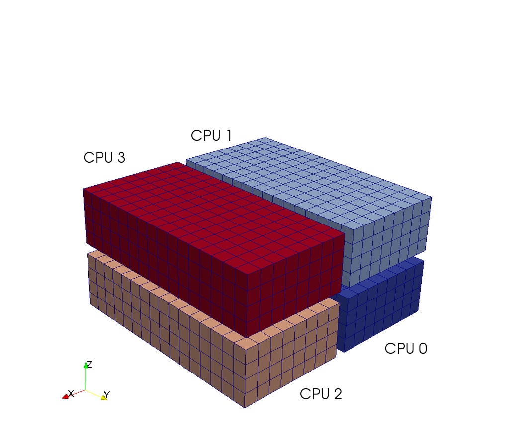
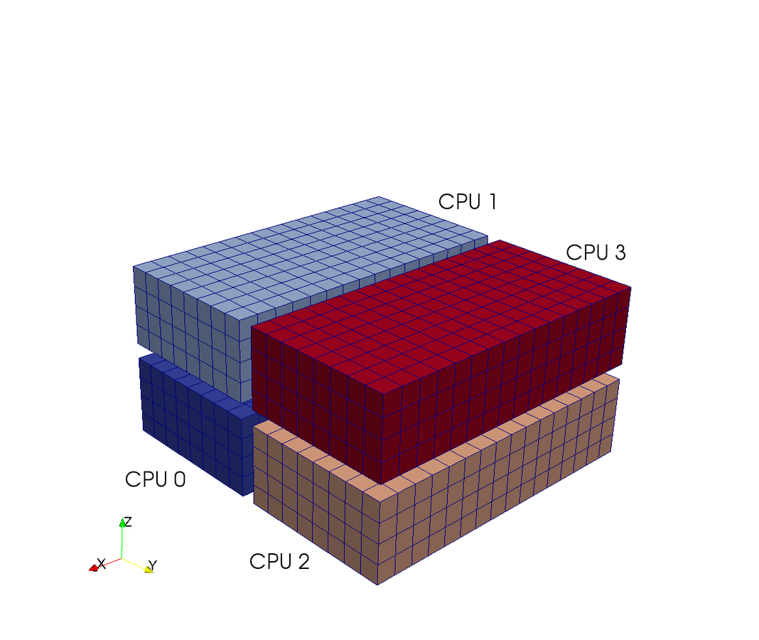
Run with MPI distribution of arrays¶

Here we would normally run from a bash shell

But since we are in a Jupyter notebook lets actually do this from python in a live cell:-)

Note that Fourier bases are especially attractive because of features easily handled with MPI:

- diagonal matrices
- fast transforms

mpi4py-fft¶

by Mikael Mortensen and Lisandro Dalcin

Highly configurable Python package for distributing multidimensional arrays and for computing fast Fourier Transforms (FFTs) in parallel. Wraps FFTW and lies at the core of shenfun and distributes large arrays.

Nonlinearities and convolutions¶

All treated with pseudo-spectral techniques. For example

$$ \begin{align} \hat{w}_k &= \widehat{\mathbf{u} \cdot \mathbf{u}}_k \\ &\text{or} \\ \hat{w}_k &= \widehat{|\nabla f|^2}_k \end{align} $$

Nonlinear terms are computed in real space and then forward transformed to spectral space.

3/2-rule or 2/3-rule possible for dealiasing of Fourier.

Mixed tensor product spaces¶

Solve several equations simultaneously

• Coupled equations
• Block matrices and vectors
• Tensor spaces of vectors, like velocity $u \in [\mathbb{R}^3]^3$

Stokes equations¶

lid-driven cavity - coupled solver¶

$$ \begin{align*} \nabla^2 \mathbf{u} - \nabla p &= \mathbf{f} \quad \text{in } \Omega, \quad \quad \Omega = [-1, 1]\times[-1, 1]\\ \nabla \cdot \mathbf{u} &= h \quad \text{in } \Omega \\ \int_{\Omega} p dx &= 0 \\ \mathbf{u}(\pm 1, y) = \mathbf{u}(x, -1) = (0, 0) &\text{ and }\mathbf{u}(x, 1) = (1, 0) \text{ or } ((1-x^2)(1+x^2), 0) \end{align*} $$

Given appropriate spaces $V$ and $Q$ a variational form reads: find $(\mathbf{u}, p) \in V \times Q$ such that

$$ \begin{equation} a((\mathbf{u}, p), (\mathbf{v}, q)) = L((\mathbf{v}, q)) \quad \forall (\mathbf{v}, q) \in V \times Q \end{equation} $$

where bilinear and linear forms are, respectively

$$ \begin{equation} a((\mathbf{u}, p), (\mathbf{v}, q)) = \int_{\Omega} (\nabla^2 \mathbf{u} - \nabla p) \cdot {\mathbf{v}} \, dx_w + \int_{\Omega} \nabla \cdot \mathbf{u} \, {q} \, dx_w, \end{equation} $$$$ \begin{equation} L((\mathbf{v}, q)) = \int_{\Omega} \mathbf{f} \cdot {\mathbf{v}}\, dx_w + \int_{\Omega} h {q} \, dx_w \end{equation} $$

Using integration by parts for Legendre (not really necessary, but looks nicer and more familiar:-)

$$ \begin{equation} a((\mathbf{u}, p), (\mathbf{v}, q)) = -\int_{\Omega} \nabla \mathbf{u} \cdot \nabla{\mathbf{v}} \, dx_w + \int_{\Omega} \nabla \cdot \mathbf{v} \, {p} \, dx_w + \int_{\Omega} \nabla \cdot \mathbf{u} \, {q} \, dx_w, \end{equation} $$

Implementation of spaces, basis functions¶

Implementation Stokes - matrices and solve¶

Block matrix M¶

$$ M = \begin{bmatrix} A[0]+A[1] & 0 & G[0] \\ 0 & A[2]+A[3] & G[1] \\ D[0] & D[1] & 0 \end{bmatrix} $$

where $D = G^T$ for the Legendre basis, making $M$ symmetric. For Chebyshev $M$ will not be symmetric.

Solver through scipy.sparse.linalg

For Navier-Stokes of the lid-driven cavity, see https://github.com/spectralDNS/shenfun/blob/master/demo/NavierStokesDrivenCavity.py

Sparsity pattern¶

$$ M = \begin{bmatrix} A[0]+A[1] & 0 & G[0] \\ 0 & A[2]+A[3] & G[1] \\ D[0] & D[1] & 0 \end{bmatrix} $$

Future work¶

• More linear algebra solvers. Most 1D bases are very good, but coupling two non-periodic directions demands more of
  • Block preconditioners
  • Uzawa solvers
  • matrix decomposition (some implemented)
  • MPI for all solvers
• Fast Legendre transforms
• Chebyshev-Legendre transforms
• Generalized Jacobi polynomials
• Cylindrical/circular domains
• Unbounded domains - Laguerre/Hermite recently added
  • Fast transforms
• Solvers for more than 2 non-periodic bases
• Domain decomposition
• Better documentation😃

Thank you for your time😃¶