Pull Data from all STOQS Databases on a Server
Opening read-only, loop through all databases on a server and produce some summary products
Docker Instructions
Install and start the software as
detailed in the README. (Note that on MacOS you will need to modify settings in your docker-compose.yml and .env files — look for comments referencing 'HOST_UID'.)
Then, from your $STOQS_HOME/docker directory start the Jupyter Notebook server - you can query from the remote database or from a copy that you've made to your local system:
Query from MBARI's master database
Start the Jupyter Notebook server pointing to MBARI's master STOQS database server. (Note: firewall rules limit unprivileged access to such resources):
docker-compose exec \
    -e DATABASE_URL=postgis://everyone:guest@kraken.shore.mbari.org:5432/stoqs \
    stoqs stoqs/manage.py shell_plus --notebook
Opening this Notebook
Following execution of the stoqs/manage.py shell_plus --notebook command a message is displayed giving a URL for you to use in a browser on your host, e.g.:
http://127.0.0.1:8888/?token=<a_token_generated_upon_server_start>
In the browser window opened to this URL navigate to this file (pull_from_all_databases.ipynb) and open it. You will then be able to execute the cells and modify the code to suit your needs.
import os

# Prevent SynchronousOnlyOperation exceptions
os.environ["DJANGO_ALLOW_ASYNC_UNSAFE"] = "true"

# Build a dictionary of all CANON Campaigns on the server and count things
from campaigns import campaigns
my_campaigns = {}
for db in campaigns:
    print(db)
    try:
        c = Campaign.objects.using(db).get(id=1)
        ##if 'simz' in db:
        if 'CANON' in c.name:
            print('{:25s} {}'.format(db, c.description))
            my_campaigns[db] = c
    except Exception as e:
        ##print('{:25s} *** {} ***'.format(db, e))
        pass
stoqs_rovctd_mb
stoqs_rovctd_mw93
stoqs_rovctd_mw97
stoqs_oceansites_o
stoqs_rovctd_goc
stoqs_september2010
stoqs_october2010
stoqs_october2010         Bloomex observing campaign in Monterey Bay
stoqs_dorado2009
stoqs_dorado2011
stoqs_april2011
stoqs_april2011           Dorado and Tethys surveys in Monterey Bay
stoqs_june2011
stoqs_june2011            Front detection Dorado and Tethys surveys in Monterey Bay
stoqs_february2012
stoqs_may2012
stoqs_may2012             Front detection AUV and Glider surveys in Monterey Bay
stoqs_september2012
stoqs_september2012       Western Flyer and Tethys following drifting ESP off of Big Sur
stoqs_ioos_gliders
stoqs_march2013
stoqs_march2013_o
stoqs_march2013_o         Spring 2013 ECOHAB in San Pedro Bay
stoqs_beds2013
stoqs_beds_canyon_events
stoqs_simz_aug2013
stoqs_september2013
stoqs_september2013       Intensive 27 platform observing campaign in Monterey Bay
stoqs_september2013_o
stoqs_cn13id_oct2013
stoqs_simz_oct2013
stoqs_simz_spring2014
stoqs_canon_april2014
stoqs_canon_april2014     Spring 2014 ECOHAB in San Pedro Bay
stoqs_simz_jul2014
stoqs_september2014
stoqs_september2014       Fall 2014 Dye Release Experiment in Monterey Bay
stoqs_simz_oct2014
stoqs_canon_may2015
stoqs_canon_may2015       Spring 2015 Experiment in Monterey Bay
stoqs_os2015
stoqs_os2015              CANON Off Season 2015 Experiment in Monterey Bay
stoqs_canon_september2015
stoqs_canon_september2015 Fall 2015 Front Identification in northern Monterey Bay
stoqs_os2016
stoqs_os2016              None
stoqs_cce2015
stoqs_michigan2016
stoqs_canon_september2016
stoqs_os2017
Collect the SimpleDepthTime data into a Pandas DataFrame so that we can plot the distribution of data over time. (Use the STOQS schema diagram to navigate the data model and construct queries.)
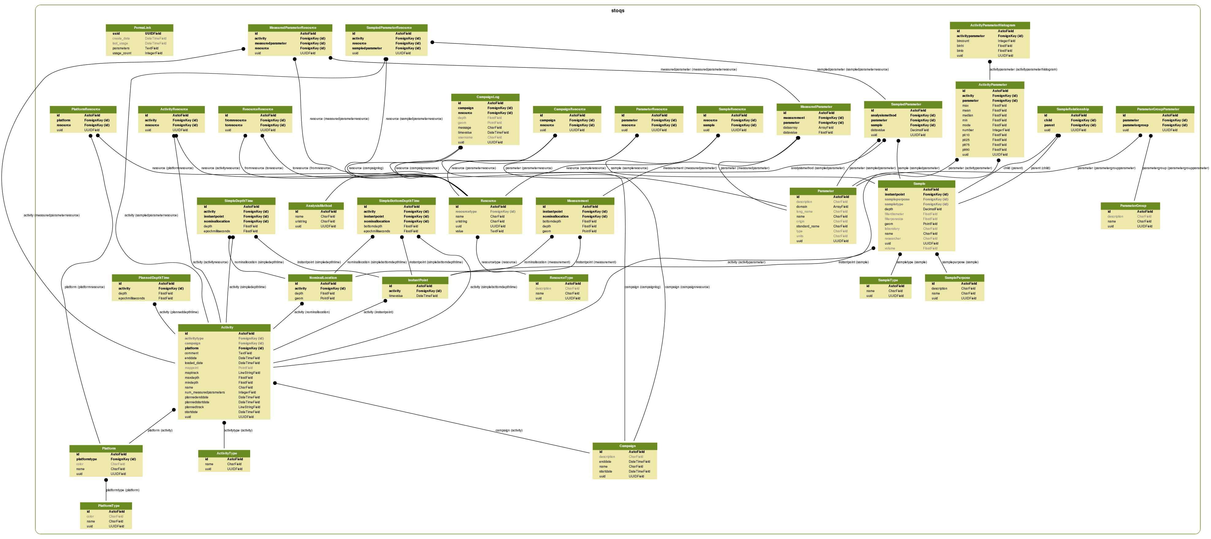
%%time
import geopandas as gpd
df = gpd.GeoDataFrame()
for db, c in my_campaigns.items():
    c_sum = 0
    if c.startdate.year > 2012:
        continue
    print(f'{db:25s}', end='')
    for platform in Platform.objects.using(db).all():
        sdtp = SimpleDepthTime.objects.using(db).filter(activity__platform=platform)
        sdtp = sdtp.order_by('instantpoint__timevalue').values('activity__name',
                                 'activity__platform__name', 'activity__platform__color',
                                 'activity__maptrack', 'instantpoint__timevalue', 'depth')
        try:
            c_sum += sdtp.count()
            p_df = gpd.GeoDataFrame.from_records(sdtp, index='instantpoint__timevalue')
        except KeyError:
            ##print "No time series of {} from ()".format(platform, db)
            pass
        df = df.append(p_df)
    print(f'{c_sum} records')
stoqs_october2010        5571 records
stoqs_april2011          9210 records
stoqs_june2011           5886 records
stoqs_may2012            10334 records
stoqs_september2012      2357 records
CPU times: user 6.66 s, sys: 864 ms, total: 7.52 s
Wall time: 45.8 s
Before plotting the platform tracks on a map we need to fix up a few things so that we can use the geodjango plotting functions.
# Monkey patch PostGIS/GEOS LineString with properties that GeoPandas's GeoSeries expects
from django.contrib.gis.geos.linestring import LineString
LineString.type = LineString.geom_type
LineString.bounds = LineString.extent

# GeoPandas default geometry column is named 'geometry'; and rename the color column
df = df.rename(columns={'activity__maptrack': 'geometry'})
df = df.rename(columns={'activity__platform__color': 'color'})

# Make our color column a value that's understood
df['color'] = '#' + df['color']
df['geometry'].values[0].bounds
(-122.08666470977943,
 36.78165528732658,
 -121.83581780436333,
 36.92574003579148)
df.dropna().total_bounds
(-127.0008, 34.450001, -121.78523883260067, 36.981701000000001)
# Download from https://www.naturalearthdata.com/downloads/10m-physical-vectors/
coast_df = gpd.GeoDataFrame.from_file('./ne_10m_coastline.shp')
%matplotlib inline
from pylab import plt
plt.style.use('ggplot')
plt.rcParams['figure.figsize'] = (18.0, 18.0)
ax = df.dropna().plot()
ax.set_autoscale_on(False)
coast_df.plot()
Plot time-depth traces of all the Platforms; similar to the STOQS UI, but for all the Campaigns
%matplotlib inline
from pylab import plt
plt.style.use('ggplot')
plt.rcParams['figure.figsize'] = (18.0, 6.0)
fig, ax = plt.subplots(1,1)
ax.set_title('All MBARI CANON Campaign Data')
ax.set_ylabel('Depth (m)')
ax.invert_yaxis()

for p, c in df.set_index('activity__platform__name'
                        )['color'].to_dict().items():
    pdf = df.loc[df['activity__platform__name'] == p]
    for a in pdf['activity__name'].unique():
        # Plot each activity individually so as not to connect them
        pdf.loc[pdf['activity__name'] == a].depth.plot(label=p, c=c)

# See http://stackoverflow.com/questions/13588920/stop-matplotlib-repeating-labels-in-legend
from collections import OrderedDict
handles, labels = plt.gca().get_legend_handles_labels()
by_label = OrderedDict(zip(labels, handles))
_ = ax.legend(by_label.values(), by_label.keys(), loc='best', ncol=4)

Make the same plot using Bokeh so that we can zoom in — when executed on your computer — and see details. (Plot does not show on GitHub.)
from bokeh.plotting import figure, show
from bokeh.io import output_notebook

fig = figure(width = 900, height = 400,
             title = 'All MBARI CANON Campaign Data',
             x_axis_type="datetime",
             x_axis_label='Time (GMT)',
             y_axis_label = 'Depth (m)')

output_notebook(hide_banner=True)

# Negate the depth values until we figure out how to invert a bokeh axis
df2 = df.copy()
df2['depth'] *= -1
for p, c in df2.set_index('activity__platform__name'
                         )['color'].to_dict().items():
    pdf = df2.loc[df['activity__platform__name'] == p]
    for a in pdf['activity__name'].unique():
        adf = pdf.loc[pdf['activity__name'] == a]['depth']
        fig.line(x=adf.index, y=adf.values, line_color=c)

_ = show(fig)
Count up all of the MeasuredParameters in the databases.
mp_total = 0
for db, c in my_campaigns.items():
    try:
        mpc = CampaignResource.objects.using(db).get(
            campaign=c, resource__name='MeasuredParameter_count')
        print('{:25s} {:-12,}'.format(db, int(mpc.resource.value)))
        mp_total += int(mpc.resource.value)
    except Exception:
        pass

print('{:25s} {:12s}'.format('', 12*'-'))
print('{:25s} {:-12,}'.format('total', mp_total))
stoqs_october2010            5,770,879
stoqs_april2011             21,729,584
stoqs_june2011              18,336,887
stoqs_september2012          1,960,329
stoqs_march2013_o            3,023,957
stoqs_september2013         40,918,813
stoqs_canon_april2014          886,583
stoqs_september2014          2,188,968
stoqs_canon_may2015          1,109,931
stoqs_os2015                   537,799
                          ------------
total                       96,463,730
About 100 million measurments to work with. Let's examine the MeasuredParameter statistics for some of the Platforms.
Define a function to get a Pandas DataFrame of statistics of the MeasuredParameters for a Platform.
import pandas as pd
def df_stats(platform):
    df = pd.DataFrame()
    for db, c in my_campaigns.items():
        aps = ActivityParameter.objects.using(db).filter(activity__platform__name=platform)
        aps = aps.values('activity__startdate', 'parameter__name', 'mean', 'p025', 'p975')
        df = df.append(pd.DataFrame.from_records(aps))

    return df
Define a function to plot a time series of the statistical values in the dataframe: mean and 2.5 & 97.5 percentiles
%matplotlib inline
from pylab import plt
plt.rcParams['figure.figsize'] = (14.0, 4.0)
plt.style.use('ggplot')
def ts_plot(df, parm):
    d = df[df['parameter__name'] == parm]
    d.plot(x='activity__startdate', marker='*')
    plt.ylabel(parm)
Get statistics for Dorado measurements
dorado_df = df_stats('dorado')
dorado_df.head()
| activity__startdate | mean | p025 | p975 | parameter__name | |
|---|---|---|---|---|---|
| 0 | 2010-10-04 21:50:01 | 11.211672 | 10.139740 | 13.040213 | temperature |
| 1 | 2010-10-04 21:50:01 | 3.851595 | 2.374692 | 6.613944 | oxygen |
| 2 | 2010-10-04 21:50:01 | 18.895955 | 4.220000 | 26.980000 | nitrate |
| 3 | 2010-10-04 21:50:01 | 0.006486 | 0.000960 | 0.015468 | bbp420 |
| 4 | 2010-10-04 21:50:01 | 0.006510 | 0.001153 | 0.015715 | bbp700 |
Plot time series of the mean and 2.5%, 97.5% values of the distribution to detect trends, patterns, or outliers in the data.
for p in dorado_df.parameter__name.unique():
    ts_plot(dorado_df, p)


Can do the same for any other platform, e.g. M1 mooring:
m1_df = df_stats('M1_Mooring')
for p in m1_df.parameter__name.unique():
    ts_plot(m1_df, p)


