 Agenda
 Additional Packages for Google Colab
If you are using Google Colab, you have to install additional packages. To do this, simply run the following cell.
# to work locally (win/linux/mac), first install 'graphviz': https://graphviz.org/download/ and restart your machine
!pip install torchviz
Collecting torchviz
  Downloading https://files.pythonhosted.org/packages/8f/8e/a9630c7786b846d08b47714dd363a051f5e37b4ea0e534460d8cdfc1644b/torchviz-0.0.1.tar.gz (41kB)
     |████████████████████████████████| 51kB 3.7MB/s
Requirement already satisfied: torch in /usr/local/lib/python3.6/dist-packages (from torchviz) (1.7.0+cu101)
Requirement already satisfied: graphviz in /usr/local/lib/python3.6/dist-packages (from torchviz) (0.10.1)
Requirement already satisfied: future in /usr/local/lib/python3.6/dist-packages (from torch->torchviz) (0.16.0)
Requirement already satisfied: dataclasses in /usr/local/lib/python3.6/dist-packages (from torch->torchviz) (0.8)
Requirement already satisfied: typing-extensions in /usr/local/lib/python3.6/dist-packages (from torch->torchviz) (3.7.4.3)
Requirement already satisfied: numpy in /usr/local/lib/python3.6/dist-packages (from torch->torchviz) (1.19.5)
Building wheels for collected packages: torchviz
  Building wheel for torchviz (setup.py) ... done
  Created wheel for torchviz: filename=torchviz-0.0.1-cp36-none-any.whl size=3522 sha256=6a736ad7c5fb8745a0b4912099f190f303604fe6b847bd2e0ab2e6141c6b5828
  Stored in directory: /root/.cache/pip/wheels/2a/c2/c5/b8b4d0f7992c735f6db5bfa3c5f354cf36502037ca2b585667
Successfully built torchviz
Installing collected packages: torchviz
Successfully installed torchviz-0.0.1
# imports for the tutorial
import numpy as np
import pandas as pd
import torch
import torch.nn as nn
import torchviz
import matplotlib.pyplot as plt
from sklearn.model_selection import train_test_split
from sklearn.linear_model import Perceptron, LogisticRegression
from sklearn.preprocessing import StandardScaler
%matplotlib inline
 Discriminative Models
- Discriminative models are a class of models used in statistical classification, especially in supervised machine learning. A discriminative classifier tries to build a model just by depending on the observed data while learning how to do the classification from the given statistics.
- Compared to generative models, discriminative models make fewer assumptions on the distributions but depend heavily on the quality of the data.
- For example, given a set of labeled pictures of dog and rabbit, discriminative models will be matching a new, unlabeled picture to a most similar labeled picture and then give out the label class, a dog or a rabbit.
- The typical discriminative learning approaches include Logistic Regression (LR), Support Vector Machine (SVM), conditional random fields (CRFs) (specified over an undirected graph), and others.
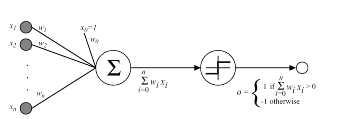
 The Perceptron
- One of the first and simplest linear model.
- Based on a linear threshold unit (LTU): the input and output are numbers (not binary values), and each connection is associated with a weight.
- The LTU computes a weighted sum of its inputs: $z = w_1x_1 + w_2x_2 +....+w_nx_n = w^Tx$, and then it applies a step function to that sum and outputs the result: $$ h_w(x) = step(z) = step(w^Tx) $$
- Illustration:
- Perceptron Training draws inspiration from biological neurons: the connection weight between two neurons is increased whenever they have the same output. Perceptrons are trained by considering the error made.
- At each iteration, the Perceptron is fed with one training instance and makes a prediction for it.
- For every output that produced a wrong prediction, it reinforces the connection weights from the inputs that would have contributed to the correct prediction.
- Criterion: $ E^{perc}(w) = - \sum_{i \in D_{miss}}w^T(x^iy^i) $
- Perceptron Learning Rule (weight update): $$ w_{t+1} = w_t +\eta(y_i -sign(w_t^Tx_i))x_i $$
- $\eta$ is the learing rate (hyper-parameter).
- The decision boundary learned is linear, the Perceptron is incapable of learning complex patterns.
- Perceptron Convergence Theorem: If the training instances are linearly seperable, the algorithm would converge to a solution.
- There can be multiple solutions (multiple hyperplanes).
- Perceptrons do not output a class probability, they just make predicitons based on a hard threshold.
- Pseudocode:
- Require: Learning rate $\eta$
- Require: Initial parameter $w$
- While stopping criterion not met do
- For $i=1,...,m$:
- $ w_{t+1} \leftarrow w_t +\eta(y_i -sign(w_t^Tx_i))x_i $
- $t \leftarrow t + 1$
- For $i=1,...,m$:
- end while
# let's load the cancer dataset, shuffle it and  speratre into train and test set
dataset = pd.read_csv('./datasets/cancer_dataset.csv')
# print the number of rows in the data set
number_of_rows = len(dataset)
num_train = int(0.8 * number_of_rows)
# reminder, the data looks like this
dataset.sample(10)
| id | diagnosis | radius_mean | texture_mean | perimeter_mean | area_mean | smoothness_mean | compactness_mean | concavity_mean | concave points_mean | ... | texture_worst | perimeter_worst | area_worst | smoothness_worst | compactness_worst | concavity_worst | concave points_worst | symmetry_worst | fractal_dimension_worst | Unnamed: 32 | |
|---|---|---|---|---|---|---|---|---|---|---|---|---|---|---|---|---|---|---|---|---|---|
| 351 | 899667 | M | 15.750 | 19.22 | 107.10 | 758.6 | 0.12430 | 0.23640 | 0.29140 | 0.12420 | ... | 24.17 | 119.40 | 915.3 | 0.15500 | 0.50460 | 0.68720 | 0.21350 | 0.4245 | 0.10500 | NaN |
| 27 | 852781 | M | 18.610 | 20.25 | 122.10 | 1094.0 | 0.09440 | 0.10660 | 0.14900 | 0.07731 | ... | 27.26 | 139.90 | 1403.0 | 0.13380 | 0.21170 | 0.34460 | 0.14900 | 0.2341 | 0.07421 | NaN |
| 568 | 92751 | B | 7.760 | 24.54 | 47.92 | 181.0 | 0.05263 | 0.04362 | 0.00000 | 0.00000 | ... | 30.37 | 59.16 | 268.6 | 0.08996 | 0.06444 | 0.00000 | 0.00000 | 0.2871 | 0.07039 | NaN |
| 535 | 919555 | M | 20.550 | 20.86 | 137.80 | 1308.0 | 0.10460 | 0.17390 | 0.20850 | 0.13220 | ... | 25.48 | 160.20 | 1809.0 | 0.12680 | 0.31350 | 0.44330 | 0.21480 | 0.3077 | 0.07569 | NaN |
| 497 | 914580 | B | 12.470 | 17.31 | 80.45 | 480.1 | 0.08928 | 0.07630 | 0.03609 | 0.02369 | ... | 24.34 | 92.82 | 607.3 | 0.12760 | 0.25060 | 0.20280 | 0.10530 | 0.3035 | 0.07661 | NaN |
| 358 | 9010333 | B | 8.878 | 15.49 | 56.74 | 241.0 | 0.08293 | 0.07698 | 0.04721 | 0.02381 | ... | 17.70 | 65.27 | 302.0 | 0.10150 | 0.12480 | 0.09441 | 0.04762 | 0.2434 | 0.07431 | NaN |
| 75 | 8610404 | M | 16.070 | 19.65 | 104.10 | 817.7 | 0.09168 | 0.08424 | 0.09769 | 0.06638 | ... | 24.56 | 128.80 | 1223.0 | 0.15000 | 0.20450 | 0.28290 | 0.15200 | 0.2650 | 0.06387 | NaN |
| 464 | 911320502 | B | 13.170 | 18.22 | 84.28 | 537.3 | 0.07466 | 0.05994 | 0.04859 | 0.02870 | ... | 23.89 | 95.10 | 687.6 | 0.12820 | 0.19650 | 0.18760 | 0.10450 | 0.2235 | 0.06925 | NaN |
| 323 | 895100 | M | 20.340 | 21.51 | 135.90 | 1264.0 | 0.11700 | 0.18750 | 0.25650 | 0.15040 | ... | 31.86 | 171.10 | 1938.0 | 0.15920 | 0.44920 | 0.53440 | 0.26850 | 0.5558 | 0.10240 | NaN |
| 485 | 913063 | B | 12.450 | 16.41 | 82.85 | 476.7 | 0.09514 | 0.15110 | 0.15440 | 0.04846 | ... | 21.03 | 97.82 | 580.6 | 0.11750 | 0.40610 | 0.48960 | 0.13420 | 0.3231 | 0.10340 | NaN |
10 rows × 33 columns
# we will take the first 2 features as our data (X) and the diagnosis as labels (y)
x = dataset[['radius_mean', 'texture_mean']].values
y = dataset['diagnosis'].values == 'M'  # 1 for Malignat, 0 for Benign
# shuffle
rand_gen = np.random.RandomState(0)
shuffled_indices = rand_gen.permutation(np.arange(len(x)))

x_train = x[shuffled_indices[:num_train]]
y_train = y[shuffled_indices[:num_train]]
x_test = x[shuffled_indices[num_train:]]
y_test = y[shuffled_indices[num_train:]]

print("total training samples: {}, total test samples: {}".format(num_train, number_of_rows - num_train))
total training samples: 455, total test samples: 114
# fit scaler on training data (not on test data!)
scaler = StandardScaler().fit(x_train)

# transform training data
x_train = scaler.transform(x_train)

# transform testing data
x_test = scaler.transform(x_test)
# perceptron using Scikit-Learn
per_clf = Perceptron(max_iter=1000)
per_clf.fit(x_train, y_train)
y_pred = per_clf.predict(x_test)
accuracy = np.sum(y_pred == y_test) / len(y_test)
print("perceptron accuracy: {:.3f} %".format(accuracy * 100))
w = (per_clf.coef_).reshape(-1,)
b = (per_clf.intercept_).reshape(-1,)
boundary = (-b -w[0] * x_train[:, 0]) / w[1]
perceptron accuracy: 85.088 %
def plot_perceptron_result():
    fig = plt.figure(figsize=(10, 8))
    ax = fig.add_subplot(1,1,1)
    ax.scatter(x_train[y_train,0], x_train[y_train, 1], color='r', label="M, train", alpha=0.5)
    ax.scatter(x_train[~y_train,0], x_train[~y_train, 1], color='b', label="B, train", alpha=0.5)
    ax.scatter(x_test[y_test,0], x_test[y_test, 1], color='r', label="M, test", alpha=1)
    ax.scatter(x_test[~y_test,0], x_test[~y_test, 1], color='b', label="B, test", alpha=1)
    ax.plot(x_train[:,0], boundary, label="decision boundary", color='g')
    ax.legend()
    ax.grid()
    ax.set_ylim([-5, 5])
    ax.set_xlabel("radius_mean")
    ax.set_ylabel("texture_mean")
    ax.set_title("texture_mean vs. radius_mean")
# plot
plot_perceptron_result()

 MLE with Bernoulli Assumption
Recall that there is a connection between maximum likelihood estimation (MLE) and linear regression when we assume that the data can be created as follows: $y=\theta^Tx + \epsilon$, where $\epsilon \sim \mathcal{N}(0, \sigma^2) \to y \sim \mathcal{N}(\theta^Tx, \sigma^2)$.
- In this case, minimizing the negative log-likelihood (NLL): $-\log P(y|x;\theta)$ results in the MSE error $(y-\theta^Tx)^2$, and minimizing the NLL is the same as maximizing $\log P(y|x;\theta)$, which is exactly the MLE!
When we assume that the data is created in a different way, we get different loss functions, as we will now demonstrate. But the idea is the same --
maximizing the log-likelihood (MLE) = minimizing the negative log-likelihood (NLL). $$ \log P(y|x;\theta) = \log \left[\frac{1}{\sqrt{2 \pi \sigma^2}} \exp{\left(-\frac{(y - \theta^Tx)^2}{2\sigma^2}\right)} \right] $$ $$ = -0.5\log(2\pi\sigma^2) -\frac{1}{2\sigma^2}(y -\theta^Tx)^2$$ $$ \to \max_{\theta}\log P(y|x;\theta) = \min_{\theta}-\log P(y|x;\theta) = \min_{\theta}\frac{1}{2}(y -\theta^Tx)^2 = \min_{\theta} MSE $$
The Sigmoid function (also the Logistic Function): $$ \sigma(x) = \frac{1}{1+e^{-x}} = \frac{e^x}{1+e^x} $$
- The output is in $[0,1]$, which is exactly what we need to model a probability distribution.
We assume that: $$ P(y|x,\theta) = Bern(y|\sigma(\theta^Tx)) $$
- Bernoulli Distribution (coin flip): $$ P(y) = p^y(1-p)^{1-y} $$
- $p = \sigma(\theta^Tx) \in [0,1]$
We will use the following notations:
# let's see the sigmoid function
def sigmoid(x):
    return 1 / (1 + np.exp(-x))

x = np.linspace(-5, 5, 1000)
sig_x = sigmoid(x)
# plot
fig = plt.figure(figsize=(8,5))
ax = fig.add_subplot(111)
ax.plot(x, sig_x)
ax.grid()
ax.set_title("The Sigmoid Function")
ax.set_xlabel("x")
ax.set_ylabel("sigmoid(x)")
Text(0, 0.5, 'sigmoid(x)')

 Logistic Regression
- Some regression algorithms can be used for classification as well.
- Logistic Regression is commonly used to estimate the probability that an instance belongs to a particular class.
- Typically, if the estimated proabibility is greater than 50%, then the model predicts that the instance belongs to that class (called the positive class, labeled "1"), or else it predicts that it does not - a binary classifier.
- Estimating Probabilities - Similarly to Linear Regression, a Logistic Regression model computes a weighted sum of the input features (plus a bias term), but unlike Linear Regression, it outputs the logistic of the weighted sum - $\sigma(w^Tx)$, which is a number between 0 and 1.
Training and Cost Function
- The objective of training is to set the parameter vector $\theta$ (or $w$) so that the model estimates high probabilities for positive instances ($y=1$) and low probabilities for negative instances ($y=0$)
- Expanding the expression using the negative log-likelihood (NLL): $$ P(y|x,\theta) = Bern(y|\sigma(\theta^Tx)) \rightarrow NLL(\theta) = -\frac{1}{m}\sum_{i=1}^m \log \sigma(\theta^Tx_i)^{y_i}(1-\sigma(\theta^Tx_i))^{1-y_i} =- \frac{1}{m} \sum_{i=1}^m\log\pi_{i1}^{y_i}\pi_{i0}^{1-y_i} $$ $$ = -\frac{1}{m} \sum_{i=1}^m \left[y_i\log\pi_{i1} + (1-y_i)\log\pi_{i0} \right]$$
- This yields the Logistic Regression cost function (log loss): $$ J(\theta) = -\frac{1}{m} \sum_{i=1}^m \big[ y_i\log \pi_{i1} + (1-y_i)\log \pi_{i0} \big] = -\frac{1}{m} \sum_{i=1}^m \big[ y_i\log \pi_{i1} + (1-y_i)\log (1 - \pi_{i1}) \big] $$
- Intuition: $-\log(t)$ grows very large when $t$ approaches 0, so the cost will be large if the model estimates a probability close to 0 for a positive instance, and it will also be very large if the estimated probability is close to 1 for a negative instance. On the other hand, $-log(t)$ is close to 0 when $t$ is close to 1, so the cost will be close to 0 if the estimated probability is close to 0 for a negative instance or close to 1 for a positive instance.
- This expression is also called the binary cross-entropy (BCE) loss.
- The cost function in the case of Logistic Regression is convex.
- Logistic cost function derivatives: $$ \frac{\partial}{\partial \theta_j}J(\theta) = \frac{1}{m}\sum_{i=1}^m \big( \sigma(\theta^Tx^{i}) - y_i \big) x_j^{i} $$
- No closed-form solution.
- Thanks to the convexity of the cost function (for the case of Logistic Regression), we can use Gradient Descent (or SGD, Mini-Batch GD).
def plot_lr_boundary(x_train, x_test, y_train, y_test, boundary):
    fig = plt.figure(figsize=(8, 5))
    ax = fig.add_subplot(1,1,1)
    ax.scatter(x_train[y_train,0], x_train[y_train, 1], color='r', label="M, train", alpha=0.5)
    ax.scatter(x_train[~y_train,0], x_train[~y_train, 1], color='b', label="B, train", alpha=0.5)
    ax.scatter(x_test[y_test,0], x_test[y_test, 1], color='r', label="M, test", alpha=1)
    ax.scatter(x_test[~y_test,0], x_test[~y_test, 1], color='b', label="B, test", alpha=1)
    ax.plot(x_train[:,0], boundary, label="decision boundary", color='g')
    ax.legend()
    ax.grid()
    ax.set_ylim([-5, 5])
    ax.set_xlabel("radius_mean")
    ax.set_ylabel("texture_mean")
    ax.set_title("texture_mean vs. radius_mean")
# logistic regression with scikit-learn
log_reg = LogisticRegression(solver='lbfgs')
log_reg.fit(x_train, y_train)
y_pred = log_reg.predict(x_test)
accuracy = np.sum(y_pred == y_test) / len(y_test)
print("Logistic Regression accuracy: {:.3f} %".format(accuracy * 100))
w = (log_reg.coef_).reshape(-1,)
b = (log_reg.intercept_).reshape(-1,)
boundary = (-b -w[0] * x_train[:, 0]) / w[1]
Logistic Regression accuracy: 90.351 %
# plot
plot_lr_boundary(x_train, x_test, y_train, y_test, boundary)

 Logistic Regression with PyTorch
- We will now get familiar with building neural networks with PyTorch.
- All neural network models inherit from a parent class
nn.Module. The user must implement the__init__()and__forward()__methods. - In
__init__()we initialize the parameters of the neural networks, e.g., number of parameters (such as number of hidden units/layers, type of layers and etc...) - In
__forward()__we implement the forward pass of the network, i.e., what happens to the input.- For example, if in
__init__()you defined a linear layer and a ReLU activation, then in__forward()__you will define that the input goes first into the linear layer and then into the activation.
- For example, if in
# define our simple single neuron network
class SingleNeuron(nn.Module):
    # notice that we inherit from nn.Module
    def __init__(self, input_dim):
        super(SingleNeuron, self).__init__()
        # here we initialize the building blocks of our network
        # single neuron is just one linear (fully-connected) layer
        self.fc = nn.Linear(input_dim, 1)
        # non-linearity: the sigmoid function for binary classification
        self.sigmoid = nn.Sigmoid()

    def forward(self, x):
        # here we define what happens to the input x in the forward pass
        # that is, the order in which x goes through the building blocks
        # in our case, x first goes through the signle neuron and then activated with sigmoid
        return self.sigmoid(self.fc(x))
- Okay, so we have our network, now we need to train it.
- We need to define how to optimize the weights and other hyper-parameters, such as number of epochs.
# define the device we are going to run calculations on (cpu or gpu)
device = torch.device("cuda:0" if torch.cuda.is_available() else "cpu")
# create an instance of our model and send it to the device
input_dim = x_train.shape[1]
model = SingleNeuron(input_dim=input_dim).to(device)
# define optimizer, and give it the networks weights
learning_rate = 0.1
# every class that inherits from nn.Module() has the .parameters() method to access the weights
optimizer = torch.optim.SGD(model.parameters(), lr=learning_rate)
# other hyper-parameters
num_epochs = 5000
# define loss function - BCE for binary classification
criterion = nn.BCELoss()
# preprocess the data
scaler = StandardScaler()
x_train_prep = scaler.fit_transform(x_train)
x_test_prep = scaler.transform(x_test)
# training loop for the model
for epoch in range(num_epochs):
    # get data
    features = torch.tensor(x_train_prep, dtype=torch.float, device=device)
    labels = torch.tensor(y_train, dtype=torch.float, device=device)
    # forward pass
    logits = model(features)
    # loss
    loss = criterion(logits.view(-1), labels)
    # backward pass
    optimizer.zero_grad()  # clean the gradients from previous iteration
    loss.backward()  # autograd backward to calculate gradients
    optimizer.step()  # apply update to the weights
    if epoch % 1000 == 0:
        print(f'epoch: {epoch} loss: {loss}')
epoch: 0 loss: 0.6858659386634827
epoch: 1000 loss: 0.26053810119628906
epoch: 2000 loss: 0.25988084077835083
epoch: 3000 loss: 0.25985535979270935
epoch: 4000 loss: 0.25985416769981384
# predict and check accuracy
test_features = torch.from_numpy(x_test_prep).float().to(device)
y_pred_logits = model(test_features).data.cpu().view(-1).numpy()
y_pred = (y_pred_logits > 0.5)
accuracy = np.sum(y_pred == y_test) / len(y_test)
print("Logistic Regression accuracy: {:.3f} %".format(accuracy * 100))
Logistic Regression accuracy: 90.351 %
Same as Scikit-Learn!
# visualize computational graph
x = torch.randn(1, input_dim).to(device)
torchviz.make_dot(model(x), params=dict(model.named_parameters()))
 Multi-Class (Multinomial) Logistic Regression - Softmax Regression
- The Logistic Regression model can be generalized to support multiple classes.
- The idea: when given an instance $x$, the Softmax Regression model first computes a score $s_k(x)$ for each class $k$, then estimates a probability of each class by applying the softmax function (normalized exponential) to the scores.
- The Softmax score for class $k$: $$ s_k(x) = \big( \theta^{(k)} \big)^T \cdot x $$
- Each class has its own dedicated parameter vector $\theta^{(k)}$, which is usually stored in a row of the parameter matrix $\Theta$.
- The Softmax Function: $$\hat{p}_k = p(y=k|x,\theta) = \sigma(s(x))_k = \frac{e^{s_k(x)}}{\sum_{j=1}^K e^{s_j(x)}} $$
- $K$ is the number of classes.
- $s(x)$ is a vector containing the scores of each class for the instance $x$.
- $\sigma(s(x))_k$ is the estimated probability that the instance $x$ belongs to class $k$ given the scores of each class for that instance.
- The Softmax Regression classifier prediction: $$\hat{y} = \underset{k}{\mathrm{argmax}} \sigma(s(x))_k = \underset{k}{\mathrm{argmax}} s_k(x) = \underset{k}{\mathrm{argmax}} \big( (\theta^{(k)})^Tx \big) $$
- Cross-Entropy cost function: $$ J(\Theta) = -\frac{1}{m} \sum_{i=1}^m \sum_{k=1}^K y_k^{(i)} \log(\hat{p}_k^{(i)}) $$
- $y_k^{(i)}$ is equal to 1 if the target class for the $i^{th}$ instance is $k$, otherwise, it is 0.
- When $K=2$ it is the BCE from the previous section.
- Cross-Entropy gradient vector for class $k$: $$ \nabla_{\theta^{(k)}}J(\Theta) = \frac{1}{m}\sum_{i=1}^m (\hat{p}_k^{(i)} - y_k^{(i)})x^{(i)} $$
- Use Gradient Descent or its variants to solve
- In Scikit-Learn:
LogisticRegression(multi_class="multinomial", solver="lbfgs", C=10)- $C$ is a regularization term: the inverse of regularization strength, smaller values specify stronger regularization.
 Activation Functions
The key change made to the Perceptron that brought upon the era of deep learning is the addition of activation functions to the output of each neuron. These allow the learning of non-linear functions. We will use three popular activation functions:
- Logistic function (sigmoid): $\sigma(z) = \frac{1}{1 + e^{-z}}$. The output is in $[0,1]$ which can be used for binary clssification or as a probability.
- Hyperbolic tangent function: $tanh(z) = 2\sigma(2z) - 1$. The output is in $[-1,1]$ which tends to make each layer's output more or less normalized at the beginning of the training (which may speed up convergence).
- ReLU (Rectified Linear Unit) function: $ReLU(z) = max(0,z)$. Continuous but not differentiable at $z=0$. However, it is the most common activation function as it is fast to compute and does not bound the output (which helps with some issues during Gradient Descent).
The activation functions derivatives (for the backpropagation):
- $\frac{d\sigma(z)}{dz} = \sigma(z)(1-\sigma(z))$
- $\frac{d tanh(z)}{dz} = 1 - tanh^2(z)$
- We define the derivative at 0 to be zero: $\frac{d ReLU(z)}{dz} = 1$ if $x>0$ else $0$
# activation functions
def sigmoid(z, deriv=False):
    output = 1 / (1 + np.exp(-1.0 * z))
    if deriv:
        return output * (1 - output)
    return output

def tanh(z, deriv=False):
    output = np.tanh(z)
    if deriv:
        return 1 - np.square(output)
    return output

def relu(z, deriv=False):
    output = z if z > 0 else 0
    if deriv:
        return 1 if z > 0 else 0
    return output
def plot_activations():
    x = np.linspace(-5, 5, 1000)
    y_sig = sigmoid(x)
    y_tanh = tanh(x)
    y_relu = list(map(lambda z: relu(z), x))
    fig = plt.figure(figsize=(8, 5))
    ax1 = fig.add_subplot(2,1,1)
    ax1.plot(x, y_sig, label='sigmoid')
    ax1.plot(x, y_tanh, label='tanh')
    ax1.plot(x, y_relu, label='relu')
    ax1.grid()
    ax1.legend()
    ax1.set_xlabel('x')
    ax1.set_ylabel('y')
    ax1.set_ylim([-2, 2])
    ax1.set_title('Activation Functions')

    y_sig_derv = sigmoid(x, deriv=True)
    y_tanh_derv = tanh(x, deriv=True)
    y_relu_derv = list(map(lambda z: relu(z, deriv=True), x))
    ax2 = fig.add_subplot(2,1,2)
    ax2.plot(x, y_sig_derv, label='sigmoid')
    ax2.plot(x, y_tanh_derv, label='tanh')
    ax2.plot(x, y_relu_derv, label='relu')
    ax2.grid()
    ax2.legend()
    ax2.set_xlabel('x')
    ax2.set_ylabel('y')
    # ax2.set_ylim([-2, 2])
    ax2.set_title('Activation Functions Derivatives')
    plt.tight_layout()
# plot
plot_activations()

 Recommended Videos
 Warning!
- These videos do not replace the lectures and tutorials.
- Please use these to get a better understanding of the material, and not as an alternative to the written material.
Video By Subject
- Pereceptron - Pereceptron
- Logistic Regression - Lecture 3 | Machine Learning (Stanford)
- Softmax Regression - Softmax Regression (C2W3L08)
- Activation Functions - Activation Functions (C1W3L06)
 Credits
- Icons made by Becris from www.flaticon.com
- Icons from Icons8.com - https://icons8.com
- Datasets from Kaggle - https://www.kaggle.com/
- Examples and code snippets were taken from "Hands-On Machine Learning with Scikit-Learn and TensorFlow"