EE 046746 - Technion - Computer Vision

Elias Nehme¶

Tutorial 07 - Homography, Alignment & Panoramas¶

Agenda

Matching Local Features
Parametric Transformations
Computing Parametric Transformations
- Affine
- Projective
RANSAC
Panorama
- Warping
- Image Blending (Feathering)
Kornia & Transformations in Deep Learning
Recommended Videos
Credits

The largest panorama in the world (2014): Mont Blanc

In2WHITE Video

In2WHITE Full Image

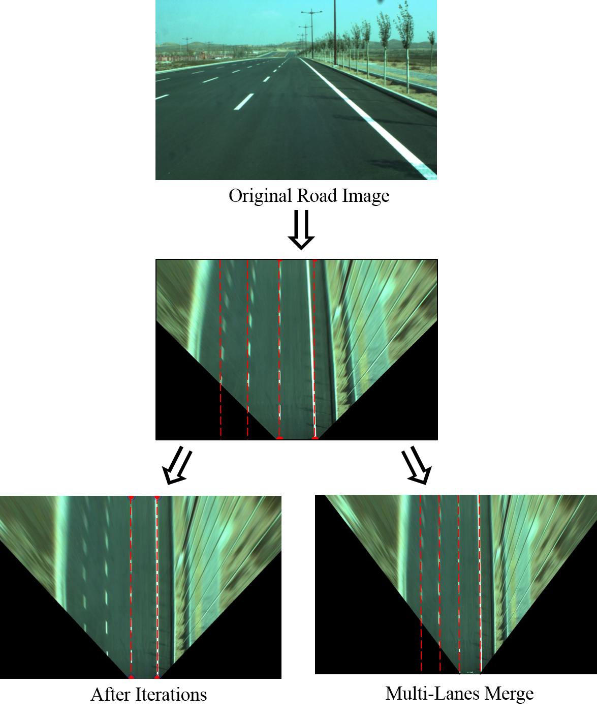
Homographic usage examples:

http://blog.flickr.net/en/2010/01/27/a-look-into-the-past/

https://www.instagram.com/albumplusart/

In [35]:

%%html
<iframe src="http://www.in2white.com/" width="700" height="600"></iframe>

In [2]:

# imports for the tutorial
import numpy as np,sys
import matplotlib.pyplot as plt
from PIL import Image
import cv2
from scipy import signal
%matplotlib inline

In [3]:

# plot images function
def plot_images(image_list, title_list, subplot_shape=(1,1), axis='off', fontsize=30, figsize=(4,4), cmap=['gray']):
    plt.figure(figsize=figsize)
    for ii, im in enumerate(image_list):
        c_title = title_list[ii]
        if len(cmap) > 1:
            c_cmap = cmap[ii]
        else:
            c_cmap = cmap[0]
        plt.subplot(subplot_shape[0], subplot_shape[1],ii+1)
        plt.imshow(im, cmap=c_cmap)
        plt.title(c_title, fontsize=fontsize)
        plt.axis(axis)

Matching Local Features

Feature matching¶

We know how to detect and describe good points
Next question: How to match them?

Typical feature matching results¶

Some matches are correct
Some matches are incorrect

Solution: search for a set of geometrically consistent matches

Parametric Transformations

Image Alignment¶

Given a set of matches, what parametric model describes a geometrically consistent transformation?

Basic 2D Transformations¶

Parametric (Global) Warping¶

Examples of parametric warps:

In [5]:

im = cv2.imread('./assets/tut_8_exm.jpg')
im = cv2.cvtColor(im,cv2.COLOR_BGR2RGB)
rows,cols,d = im.shape
print(im.shape)

# Translation:
tx,ty = [10,20]
h_T = np.float32([[1,0,tx],[0,1,ty],[0,0,1]])

# Rotation
theta = np.deg2rad(20)
h_R = np.float32([[np.cos(theta),-np.sin(theta),0],[np.sin(theta),np.cos(theta),0],[0,0,1]])

# Affine
h_AFF = np.array([[  1.26666667,-0.5,-60],[ -0.33333333,1,66.66666667],[0,0,1]])

H = [h_T,h_R,h_AFF]

img = [im]
for h in H:
    img.append(cv2.warpPerspective(im, h,(cols,rows)))
Titles = ['Original','Translation','Rotation','Affine']

# Perspective
pts1 = np.float32([[100,77],[320,105],[100,150],[385,170]])
pts2 = np.float32([[0,0],[300,0],[0,100],[300,50]])
M = cv2.getPerspectiveTransform(pts1,pts2)
im_perspective = cv2.warpPerspective(im,M,(400,300))

# Cylindrical (non linear)
def cylindricalWarp(img, K):
    """This function returns the cylindrical warp for a given image and intrinsics matrix K"""
    h_,w_ = img.shape[:2]
    # pixel coordinates
    y_i, x_i = np.indices((h_,w_))
    X = np.stack([x_i,y_i,np.ones_like(x_i)],axis=-1).reshape(h_*w_,3) # to homog
    Kinv = np.linalg.inv(K) 
    X = Kinv.dot(X.T).T # normalized coords
    # calculate cylindrical coords (sin\theta, h, cos\theta)
    A = np.stack([np.sin(X[:,0]),X[:,1],np.cos(X[:,0])],axis=-1).reshape(w_*h_,3)
    B = K.dot(A.T).T # project back to image-pixels plane
    # back from homog coords
    B = B[:,:-1] / B[:,[-1]]
    # make sure warp coords only within image bounds
    B[(B[:,0] < 0) | (B[:,0] >= w_) | (B[:,1] < 0) | (B[:,1] >= h_)] = -1
    B = B.reshape(h_,w_,-1)
    
    img_rgba = cv2.cvtColor(img,cv2.COLOR_RGB2RGBA) #BGR2BGRA for transparent borders...
    # warp the image according to cylindrical coords
    return cv2.remap(img_rgba, B[:,:,0].astype(np.float32), B[:,:,1].astype(np.float32),
                     cv2.INTER_AREA, borderMode=cv2.BORDER_TRANSPARENT)
# Camera parameters:
K = np.array([[200,0,cols/2],[0,400,rows/2],[0,0,1]]) # mock intrinsics
img_cyl = cylindricalWarp(im, K)

(362, 484, 3)

In [6]:

plot_images(img,Titles,(1,4),figsize=(16,4),fontsize=20)

plt.figure(figsize=(12,4))
plt.subplot(131)
plt.imshow(im),plt.title('Perspective input',fontsize=20)
plt.plot(pts1[:,0],pts1[:,1],'m*')
plt.axis('off')
plt.subplot(132),plt.imshow(im_perspective),plt.title('Perspective',fontsize=20)
plt.plot(pts2[:,0],pts2[:,1],'m*')
plt.axis('off')
plt.subplot(133),plt.imshow(img_cyl)
plt.title('Cylindrical',fontsize=20)
_ = plt.axis('off')

Code source - OpenCV
Cylinder code source - More Than Technical
Cylinder coordinates

Basic 2D Transformations

Basic 2D Transformations - Translation¶

$$ \begin{bmatrix} x' \\ y' \\ 1 \end{bmatrix} = \begin{bmatrix} 1 & 0 & t_x\\ 0 & 1 & t_y \\ 0 & 0 & 1 \end{bmatrix} \begin{bmatrix} x \\ y \\ 1 \end{bmatrix} = \begin{bmatrix} x+t_x \\ y+t_y \\ 1 \end{bmatrix}$$

In [11]:

# Translation:
tx,ty = [10,20]
h_T = np.float32([[1,0,tx],[0,1,ty],[0,0,1]])
im_T = cv2.warpPerspective(im, h_T,(cols,rows))

plot_images([img[0],img[1]],[Titles[0],Titles[1]],(1,2),figsize=(12,12),fontsize=20)

Basic 2D Transforation - Rotation¶

$$ \begin{bmatrix} x' \\ y' \\ 1 \end{bmatrix} = \begin{bmatrix} cos(\theta) & -sin(\theta) & 0\\sin(\theta) & cos(\theta) & 0 \\0 & 0 & 1 \end{bmatrix} \begin{bmatrix} x \\ y \\ 1 \end{bmatrix} $$

Around which point do we rotate the image?

In [12]:

# Rotation:
theta = np.deg2rad(20)
h_R = np.float32([[np.cos(theta),-np.sin(theta),0],[np.sin(theta),np.cos(theta),0],[0,0,1]])
im_R = cv2.warpPerspective(im, h_R,(cols,rows))

plot_images([img[0],img[2]],[Titles[0],Titles[2]],(1,2),figsize=(12,12),fontsize=20)

Basic 2D Transformations – Translation and Rotation (2D rigid body motion)¶

$$ \begin{bmatrix} x' \\ y' \\ 1 \end{bmatrix} = \begin{bmatrix} \cos(\theta) & -\sin(\theta) & t_x\\ \sin(\theta) & \cos(\theta) & t_y \\ 0 & 0 & 1 \end{bmatrix} \begin{bmatrix} x \\ y \\ 1 \end{bmatrix} $$

Euclidean distances are preserved
Combination of rotation and translation, which one applied first?

In [13]:

H = h_T @ h_R
im_temp = cv2.warpPerspective(im, H, (cols, rows))
plot_images([img[0], im_temp], [Titles[0], 'Rigid'], (1,2), figsize=(12,12), fontsize=20)

Basic 2D Transformations – Scale¶

$$ \begin{bmatrix} x' \\ y' \\ 1 \end{bmatrix} = \begin{bmatrix} s & 0 & 0\\ 0 & s & 0 \\ 0 & 0 & 1 \end{bmatrix} \begin{bmatrix} x \\ y \\ 1 \end{bmatrix} $$

In [14]:

# scaling
s = 1.5
h_s = np.array([[s, 0, 0], [0, s, 0], [0, 0, 1]],np.float32)
im_s = cv2.warpPerspective(im, h_s, (cols, rows))

plot_images([img[0], im_s],[Titles[0],'Scale'], (1, 2), figsize=(12,12), fontsize=20)

Basic 2D Transformations – Similarity¶

Similarity transform (4 DoF) = translation + rotation + scale

In [15]:

h_sim =  h_s @ h_T @ h_R 
im_sim = cv2.warpPerspective(im, h_sim, (cols, rows))

plot_images([img[0], im_sim], [Titles[0], 'Similarity'], (1,2), figsize=(12,12), fontsize=20)

Basic 2D Transformation - Aspect Ratio¶

$$ \begin{bmatrix} x' \\ y' \\ 1 \end{bmatrix}= \begin{bmatrix} a & 0 & 0\\ 0 & \frac{1}{a} & 0 \\ 0 & 0 & 1 \end{bmatrix} \begin{bmatrix} x \\ y \\ 1 \end{bmatrix} $$

In [16]:

# Aspect Ratio
a = 1 / 2
h_ar = np.array([[a, 0, 0], [0, 1 / a, 0], [0, 0, 1]], np.float32)
im_ar = cv2.warpPerspective(im, h_ar, (cols,rows))

plot_images([img[0], im_ar], [Titles[0], 'Aspect Ratio'], (1,2), figsize=(12,12), fontsize=20)

Basic 2D Transformations – Shear¶

$$ \begin{bmatrix} x' \\ y' \\ 1 \end{bmatrix} = \begin{bmatrix} 1 & a & 0\\ b & 1 & 0 \\ 0 & 0 & 1 \end{bmatrix} \begin{bmatrix} x \\ y \\ 1 \end{bmatrix} $$

In [17]:

# shear
a,b = (0.5, 0.1)
h_sh = np.array([[1, a, 0],[b, 1, 0], [0, 0, 1]], np.float32)
im_sh = cv2.warpPerspective(im, h_sh, (cols, rows))

plot_images([img[0], im_sh], [Titles[0], 'Shear'], (1,2), figsize=(12,12), fontsize=20)

Basic 2D Transformations – Affine¶

Similarity transform (6 DoF) = translation + rotation + scale + aspect ratio +shear

In [18]:

# affine transform
h_aff =  h_ar @ h_sh  @ h_s @ h_T @ h_R 
im_aff = cv2.warpPerspective(im, h_aff, (cols * 4, rows * 4))

plot_images([img[0], im_aff], [Titles[0], 'Affine'], (1,2), figsize=(12,12), fontsize=20)

Simple fitting procedure (linear least squares)
Approximates viewpoint change for roughly planar objects and roughly orthographic camera
Can be used to initialize fitting for more complex models

Basic 2D Transformations – Projective - a.k.a - Homographic¶

$$ \begin{bmatrix} u \\ v \\ w \end{bmatrix} = \begin{bmatrix} h_1 & h_2 & h_3\\ h_4 & h_5 & h_6 \\ \color{red}{\text{h}}_\color{red}{\text{7}} & \color{red} {\text{h}}_\color{red}{\text{8}} & 1 \end{bmatrix} \begin{bmatrix} x \\ y \\ 1 \end{bmatrix} $$$$x' = u/w$$$$y' = v/w$$

Non-linear!

In [19]:

# Perspective
pts1 = np.float32([[100,77],[320,105],[100,150],[385,170]])
pts2 = np.float32([[0,0],[300,0],[0,100],[300,50]])
h_per = cv2.getPerspectiveTransform(pts1,pts2)
im_perspective = cv2.warpPerspective(im,h_per,(400,300))

plot_images([img[0], im_perspective], [Titles[0], 'Projective'], (1, 2), figsize=(12,12), fontsize=20)

When do we get Homography?¶

Homography maps between:

points on a plane in the world and their positions in an image
points in two different images of the same plane
two images of a 3D object where the camera has rotated but not translated

For far away objects:

works fine for small viewpoint changes

Computing Affine Transformation¶

Assuming we know correspondences, how do we get transformation?

$$ \begin{bmatrix} x_i' \\ y_i' \\ 1 \end{bmatrix}= \begin{bmatrix} h_1 & h_2 & h_3\\ h_4 & h_5 & h_6 \\ 0 & 0 & 1 \end{bmatrix} \begin{bmatrix} x_i \\ y_i \\ 1 \end{bmatrix}$$$$ \begin{bmatrix} \dots \\ x_i' \\ y_i' \\ \dots \end{bmatrix}= \begin{bmatrix} &&\dots\\ x_i & y_i & 1 & 0 & 0 & 0 \\ 0&0&0&x_i&y_i&1 \\ &&\dots \end{bmatrix} \begin{bmatrix} h_1\\h_2\\h_3\\ h_4 \\ h_5 \\ h_6 \\ \end{bmatrix} $$$$b = Ah$$

Solve with Least-squares $||Ah-b||^2$ $$h = (A^TA)^{-1}A^Tb$$

In Python:

A_inv = pinv(A)

h = np.linalg.pinv(A)@b

How many matches (correspondence pairs) do we need to solve?
Once we have solved for the parameters, how do we compute the coordinates of the cooresponding point for any pixel $(x_{new},y_{new})$?

$$ H = \begin{bmatrix} h_1 & h_2 & h_3\\ h_4 & h_5 & h_6 \\ 0 & 0 & 1 \end{bmatrix} $$$$x'_{new} = Hx_{new}$$

Computing Projective Transformation¶

Recall working with homogenous coordinates

$$ \begin{bmatrix} u_i \\ v_i \\ w_i \end{bmatrix}= \begin{bmatrix} h_1 & h_2 & h_3\\ h_4 & h_5 & h_6 \\ h_7 & h_8 & 1 \end{bmatrix} \begin{bmatrix} x_i \\ y_i \\ 1 \end{bmatrix} $$$$ x_i' = u_i/w_i$$$$y_i' = v_i/w_i$$

We get the following non-linear equation:

$$ x_i' = \frac{h_1x_i + h_2 y_i + h_3}{h_7x_i+h_8y_i+h_9}$$$$y_i' = \frac{h_4x_i + h_5 y_i + h_6}{h_7x_i+h_8y_i+h_9}$$

We can re-arrange the equation

$$ \begin{bmatrix} &&&&&\dots\\ x_i & y_i & 1 & 0 & 0 & 0 & -x_ix_i'&-y_ix_i'& -x_i' \\ 0&0&0&x_i&y_i&1 & -x_iy_i'&-y_iy_i'& -y_i' \\ &&&&&\dots \end{bmatrix} \begin{bmatrix} h_1\\h_2\\h_3\\ h_4 \\ h_5 \\ h_6 \\ h_7\\h_8\\h_9\\ \end{bmatrix} = \begin{bmatrix} \dots \\ 0 \\ 0 \\ \dots \end{bmatrix}$$

We want to find a vector $h$ satisfying

$$Ah=0$$

where A is full rank. We are obviously not interested in the trivial solution $h=0$ hence we add the constraint $$||h||=1$$

Thus, we get the homogeneous Least square equation:

$$ arg\min_h{||Ah||_2^2} \text{, } s.t ||h||_2^2=1 $$

Compute Projective transformation using SVD: $$arg \min_h{||Ah||_2^2} \text{, } s.t ||h||_2^2=1 $$

Let decompose $A$ using SVD: $ A = UDV^T $, where $U$ and $V$ are orthonomal matrix, and $D$ is a diagonal matrix.
- Need a reminder on SVD? Click Here

From orthonormality of $U$ and $V$:

$$ ||UDV^Th||=||DV^Th||$$$$ ||V^Th||=||h|| $$

Hence, we get the following minimization problem:

$$ arg \min_h||DV^Th|| \text{ s.t. } ||V^Th||=1 $$

Subsitute $y=V^Th$:

$$ arg \min_h||Dy|| \text{ s.t. } ||y||=1 $$

$D$ is a diagonal matrix with decreasing values. Then, it is clear that $y=[0,0,\dots,1]^T$.

Therefore, choosing $h$ to be the last column in $V$ will minimize the equation.

In Python:

(U,D,Vh) = np.linalg.svd(A,False)

h = Vh.T[:,-1]

Some more options to find $h$:¶

Lagrange multipliers - Least–squares Solution of Homogeneous Equations
Using EVD (eigenvalue decomposition) on $A^TA$.
If we know our transformation is nearly Affine we can get an approximate solution using linear least squares

RANSAC

The RANSAC algorithm is extremly simple, but it often

Does not produce correct model with user-defined probability
Outputs an inaccurate model
Does not handle degeneracies
Can be sped up (by orders of magnitude)
Does not gurantee minimum running time
Needs information about scale of the noise
Does not handle multiple models efficiently

Many improved algorithms:

PROSAC
- Key idea is to use to assume that the similarity measure predicts correctness of a match
Randomized RANSAC
- Each step take a random subset of the query points and perform RANSAC
KALMANSAC
and more...
Estimating homogrpahy with RANSAC in OpenCV: cv2.findHomography(src_pts, dst_pts, cv2.RANSAC)

Cool application 1: Planting images into other images¶

result achieved with inverse warping and an affine transform

Cool application 2: BirdEye¶

Image Source

Cool application 3: Looking into the past¶

result achieved with inverse warping and a homography
Image Source from Flickr

Panorama

Warping
Image Blending (Feathering)

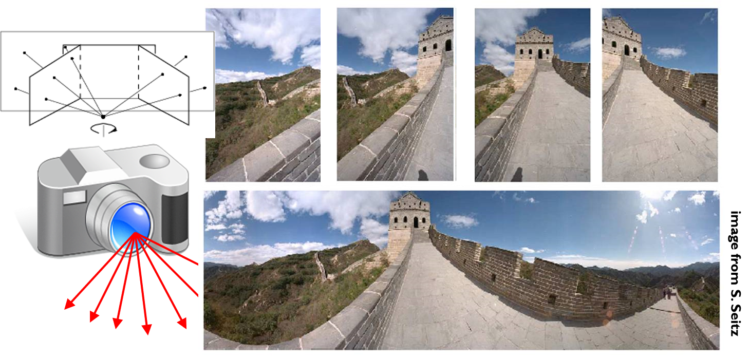
Obtain a wider angle view by combining multiple images

Warp - What we need to solve?

Given source and target images, and the transformation between them, how do we align them?
Send each pixel $x$ in image1 to its corresponding location $x’$ in image 2

Forward Warping¶

What if pixel lands “between” two pixels?
Answer: add “contribution” to several pixels and normalize (splatting)

Limitation: Holes (some pixels are never visited)

Inverse Warping¶

For each pixel x’ in image 2 find its origin x in image 1
Problem: What if pixel comes from “between” two pixels?

Answer: interpolate color value from neighbors

Bilinear Interpolation¶

Sampling at $f(x,y)$:

$$ f(x,y) = (1-a)(1-b) f[i,j]\\ + a(1-b) f[i+1,j]\\ + ab f[i+1,j+1]\\ +(1-a)b f[i,j+1]\\ $$

Python:

interp2d() - https://docs.scipy.org/doc/scipy/reference/generated/scipy.interpolate.interp2d.html
Inverse warping in OpenCV: cv2.warpPerspective(im,*,*,cv2.WARP_INVERSE_MAP)

In [20]:

import numpy as np
from scipy import interpolate
import matplotlib.pyplot as plt

x = np.arange(-5.01, 5.01, 0.25)
y = np.arange(-5.01, 5.01, 0.25)
xx, yy = np.meshgrid(x, y)
z = np.sin(xx**2+yy**2)

## Cubic
f = interpolate.interp2d(x, y, z, kind='cubic')

xnew = np.arange(-5.01, 5.01, 1e-2)
ynew = np.arange(-5.01, 5.01, 1e-2)
znew = f(xnew, ynew)


plt.figure()
plt.subplot(121)
plt.imshow(z,vmin=-1,vmax=1)
plt.subplot(122)
plt.imshow(znew,vmin=-1,vmax=1)
plt.show()

plt.figure()
plt.plot(x, z[0, :], 'ro-', xnew, znew[0, :], 'b-')
plt.show()

##linear
f = interpolate.interp2d(x, y, z, kind='linear')

xnew = np.arange(-5.01, 5.01, 1e-2)
ynew = np.arange(-5.01, 5.01, 1e-2)
znew = f(xnew, ynew)


plt.figure()
plt.subplot(121)
plt.imshow(z,vmin=-1,vmax=1)
plt.subplot(122)
plt.imshow(znew,vmin=-1,vmax=1)
plt.show()

plt.figure()
plt.plot(x, z[0, :], 'ro-', xnew, znew[0, :], 'b-')
plt.show()

Image Blending

Alpha blending
Pyramid blending

Alpha Blending¶

Pyramid Blending:¶

Build a Gaussian pyramid for each image
Build the Laplacian pyramid for each image
Decide/find the blending border (in the example: left half belongs to image 1, and right half to image 2 -> the blending border is cols/2)
- Split by index, or
- Split using a 2 masks (can be weighted masks)
Constract a new mixed pyramid - mix each level seperatly acording to (3)
Reconstract a blend image from the mixed pyramid

In [21]:

def create_pyrs(A,B):
    # generate Gaussian pyramid for A
    G = A.copy()
    gpA = [G]
    for i in range(6):
        G = cv2.pyrDown(G)
        gpA.append(G)
    # generate Gaussian pyramid for B
    G = B.copy()
    gpB = [G]
    for i in range(6):
        G = cv2.pyrDown(G)
        gpB.append(G)
    # generate Laplacian Pyramid for A
    lpA = [gpA[5]]
    for i in range(5,0,-1):
        GE = cv2.pyrUp(gpA[i])
        L = cv2.subtract(gpA[i-1],GE)
        lpA.append(L)
    # generate Laplacian Pyramid for B
    lpB = [gpB[5]]
    for i in range(5,0,-1):
        GE = cv2.pyrUp(gpB[i])
        L = cv2.subtract(gpB[i-1],GE)
        lpB.append(L)
    return lpA,lpB

def blend_images(A,B):
    lpA,lpB = create_pyrs(A,B)
    # Now add left and right halves of images in each level
    LS = []
    for la,lb in zip(lpA,lpB):
        rows,cols,dpt = la.shape
        ls = np.hstack((la[:,0:int(cols/2)], lb[:,int(cols/2):])) #mixing can also be done with a mask
        LS.append(ls)
    # now reconstruct
    ls_ = LS[0]
    for i in range(1,6):
        ls_ = cv2.pyrUp(ls_)
        ls_ = cv2.add(ls_, LS[i])
    # image with direct connecting each half
    real = np.hstack((A[:,:int(cols/2)],B[:,int(cols/2):])) 
    return real, ls_

def switch_texture(A,B):
    lpA,lpB = create_pyrs(A,B)
    # Now add left and right halves of images in each level
    LS = []
#     for la,lb in zip(lpA,lpB):
#         rows,cols,dpt = la.shape
#         ls = np.hstack((la[:,0:int(cols/2)], lb[:,int(cols/2):])) #mixing can also be done with a mask
#         LS.append(ls)
    # now reconstruct
    ls_ = lpA[0]
    for i in range(1,6):
        ls_ = cv2.pyrUp(ls_)
        ls_ = cv2.add(ls_, lpB[i])
    # image with direct connecting each half
    real = np.hstack((A[:,:int(cols/2)],B[:,int(cols/2):])) 
    return real, ls_

def alpha_blend(A,B,MASK):
    A = np.float32(A)
    B = np.float32(B)
    return np.uint8(A*MASK), np.uint8(A*MASK+B*(1-MASK))

In [22]:

A = cv2.imread('./assets/apple.jpg')
B = cv2.imread('./assets/orange.jpg')
real,ls_ = blend_images(A,B)

ls_ = cv2.cvtColor(ls_,cv2.COLOR_BGR2RGB)
real = cv2.cvtColor(real,cv2.COLOR_BGR2RGB)

In [23]:

plot_images([real,ls_],['Original','Pyramid Blend'],(1,2),figsize=(12,12),fontsize=20)

Alpha blending example:

In [24]:

MASK = np.ones_like(A,np.float32)
rows,cols,dpt = MASK.shape
w=20
v_dec = np.linspace(1,0,2*w)
MASK[:,int(cols/2):]=0
MASK[:,(int(cols/2)-w):(int(cols/2)+w)]=np.tile(np.reshape(v_dec,[1,-1,1]),[rows,1,3])
real,ls_ = alpha_blend(A,B,MASK)
ls_ = cv2.cvtColor(ls_,cv2.COLOR_BGR2RGB)
real = cv2.cvtColor(real,cv2.COLOR_BGR2RGB)

In [25]:

plot_images([real,MASK,ls_],['Original','Mask','Alpha Blending'],(1,3),figsize=(18,12),fontsize=20)

Stylize image using pyramids:

In [26]:

real,ls_ = switch_texture(A,B)
ls_ = cv2.cvtColor(ls_,cv2.COLOR_BGR2RGB)
real = cv2.cvtColor(real,cv2.COLOR_BGR2RGB)

In [27]:

plot_images([real,ls_],['Original','Texture'],(1,2),figsize=(12,12),fontsize=20)

Blending Improvments

Many algorithms have different variations of combining alpha and pyramid blending (different masks for different frequencies)
Find the boundaries using segmentation

Panorama - Summary

Detect features
Compute transformations between pairs of frames
Can Refine transformations using RANSAC
Warp all images onto a single coordinate system
Find mixing borders (e.g. using segmentation)
Blend

Transformations in Deep Learning

Can we incorporate transformations in the pipeline of a deep learning algorithm?
- Moreover, can we accelerate these transformations by performing them on a GPU?
YES!

Kornia - Computer Vision Library for PyTorch¶

Kornia is a differentiable computer vision library for PyTorch
- That means you can have gradients for the transformations!
Inspired by OpenCV, this library is composed by a subset of packages containing operators that can be inserted within neural networks to train models to perform image transformations, epipolar geometry, depth estimation, and low-level image processing such as filtering and edge detection that operate directly on tensors.
Check out kornia.geometry - https://kornia.readthedocs.io/en/latest/geometry.html
Warp image using perspective transform

Credits

EE 046746 Spring 2020 - Dahlia Urbach
Slides - Elad Osherov (Technion), Simon Lucey (CMU)
Multiple View Geometry in Computer Vision - Hartley and Zisserman - Section 2
Least–squares Solution of Homogeneous Equations - Center for Machine Perception - Tomas Svoboda
Computer vision: models, learning and inference , Simon J.D. Prince - Section 15.1
Computer Vision: Algorithms and Applications - Richard Szeliski - Sections 2,4,6, 9 (Free for Technion students via remote library)
Icons from Icon8.com - https://icons8.com