Copyright 2020 The TensorFlow Authors.
#@title Licensed under the Apache License, Version 2.0 (the "License");
# you may not use this file except in compliance with the License.
# You may obtain a copy of the License at
#
# https://www.apache.org/licenses/LICENSE-2.0
#
# Unless required by applicable law or agreed to in writing, software
# distributed under the License is distributed on an "AS IS" BASIS,
# WITHOUT WARRANTIES OR CONDITIONS OF ANY KIND, either express or implied.
# See the License for the specific language governing permissions and
# limitations under the License.
TensorFlow Profiler: Profile model performance
|
|
|
 View source on GitHub View source on GitHub
|
Overview
Machine learning algorithms are typically computationally expensive. It is thus vital to quantify the performance of your machine learning application to ensure that you are running the most optimized version of your model. Use the TensorFlow Profiler to profile the execution of your TensorFlow code.
Setup
from datetime import datetime
from packaging import version

import os
The TensorFlow Profiler requires the latest versions of TensorFlow and TensorBoard (>=2.2).
!pip install -U tensorboard_plugin_profile
WARNING: Skipping tensorflow as it is not installed.
WARNING: Skipping tensorboard as it is not installed.
     |████████████████████████████████| 517.1MB 31kB/s
     |████████████████████████████████| 2.9MB 50.9MB/s
     |████████████████████████████████| 1.1MB 61.2MB/s
     |████████████████████████████████| 460kB 61.8MB/s
import tensorflow as tf

print("TensorFlow version: ", tf.__version__)
TensorFlow version: 2.2.0-dev20200405
Confirm that TensorFlow can access the GPU.
device_name = tf.test.gpu_device_name()
if not device_name:
  raise SystemError('GPU device not found')
print('Found GPU at: {}'.format(device_name))
Found GPU at: /device:GPU:0
Train an image classification model with TensorBoard callbacks
In this tutorial, you explore the capabilities of the TensorFlow Profiler by capturing the performance profile obtained by training a model to classify images in the MNIST dataset.
Use TensorFlow datasets to import the training data and split it into training and test sets.
import tensorflow_datasets as tfds
tfds.disable_progress_bar()
(ds_train, ds_test), ds_info = tfds.load(
    'mnist',
    split=['train', 'test'],
    shuffle_files=True,
    as_supervised=True,
    with_info=True,
)
WARNING:absl:Dataset mnist is hosted on GCS. It will automatically be downloaded to your
local data directory. If you'd instead prefer to read directly from our public
GCS bucket (recommended if you're running on GCP), you can instead set
data_dir=gs://tfds-data/datasets.
Downloading and preparing dataset mnist/3.0.0 (download: 11.06 MiB, generated: Unknown size, total: 11.06 MiB) to /root/tensorflow_datasets/mnist/3.0.0...
Dataset mnist downloaded and prepared to /root/tensorflow_datasets/mnist/3.0.0. Subsequent calls will reuse this data.
Preprocess the training and test data by normalizing pixel values to be between 0 and 1.
def normalize_img(image, label):
  """Normalizes images: `uint8` -> `float32`."""
  return tf.cast(image, tf.float32) / 255., label

ds_train = ds_train.map(normalize_img)
ds_train = ds_train.batch(128)
ds_test = ds_test.map(normalize_img)
ds_test = ds_test.batch(128)
Create the image classification model using Keras.
model = tf.keras.models.Sequential([
  tf.keras.layers.Flatten(input_shape=(28, 28, 1)),
  tf.keras.layers.Dense(128,activation='relu'),
  tf.keras.layers.Dense(10, activation='softmax')
])
model.compile(
    loss='sparse_categorical_crossentropy',
    optimizer=tf.keras.optimizers.Adam(0.001),
    metrics=['accuracy']
)
Create a TensorBoard callback to capture performance profiles and call it while training the model.
# Create a TensorBoard callback
logs = "logs/" + datetime.now().strftime("%Y%m%d-%H%M%S")

tboard_callback = tf.keras.callbacks.TensorBoard(log_dir = logs,
                                                 histogram_freq = 1,
                                                 profile_batch = '500,520')

model.fit(ds_train,
          epochs=2,
          validation_data=ds_test,
          callbacks = [tboard_callback])
Epoch 1/2
469/469 [==============================] - 11s 22ms/step - loss: 0.3684 - accuracy: 0.8981 - val_loss: 0.1971 - val_accuracy: 0.9436
Epoch 2/2
 50/469 [==>...........................] - ETA: 9s - loss: 0.2014 - accuracy: 0.9439WARNING:tensorflow:From /usr/local/lib/python3.6/dist-packages/tensorflow/python/ops/summary_ops_v2.py:1271: stop (from tensorflow.python.eager.profiler) is deprecated and will be removed after 2020-07-01.
Instructions for updating:
use `tf.profiler.experimental.stop` instead.
WARNING:tensorflow:From /usr/local/lib/python3.6/dist-packages/tensorflow/python/ops/summary_ops_v2.py:1271: stop (from tensorflow.python.eager.profiler) is deprecated and will be removed after 2020-07-01.
Instructions for updating:
use `tf.profiler.experimental.stop` instead.
469/469 [==============================] - 11s 24ms/step - loss: 0.1685 - accuracy: 0.9525 - val_loss: 0.1376 - val_accuracy: 0.9595
<tensorflow.python.keras.callbacks.History at 0x7f23919a6a58>
Use the TensorFlow Profiler to profile model training performance
The TensorFlow Profiler is embedded within TensorBoard. Load TensorBoard using Colab magic and launch it. View the performance profiles by navigating to the Profile tab.
# Load the TensorBoard notebook extension.
%load_ext tensorboard
The performance profile for this model is similar to the image below.
# Launch TensorBoard and navigate to the Profile tab to view performance profile
%tensorboard --logdir=logs
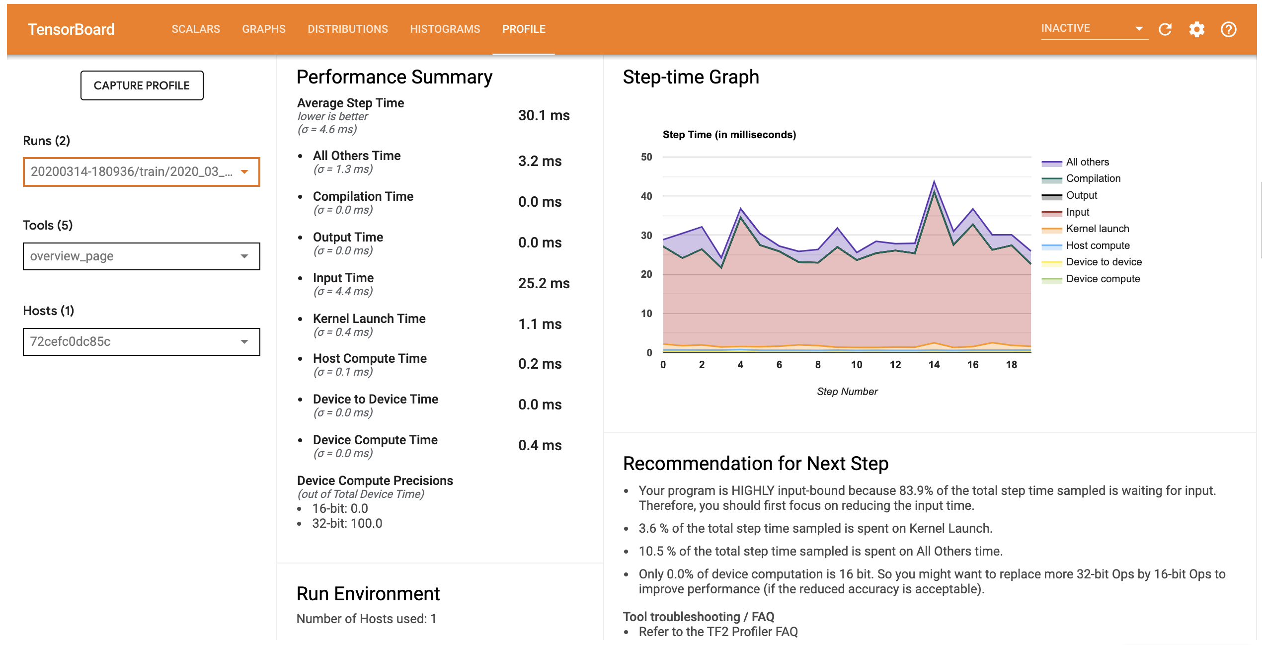
The Profile tab opens the Overview page which shows you a high-level summary of your model performance. Looking at the Step-time Graph on the right, you can see that the model is highly input bound (i.e., it spends a lot of time in the data input piepline). The Overview page also gives you recommendations on potential next steps you can follow to optimize your model performance.
To understand where the performance bottleneck occurs in the input pipeline, select the Trace Viewer from the Tools dropdown on the left. The Trace Viewer shows you a timeline of the different events that occured on the CPU and the GPU during the profiling period.
The Trace Viewer shows multiple event groups on the vertical axis. Each event group has multiple horizontal tracks, filled with trace events. The track is an event timeline for events executed on a thread or a GPU stream. Individual events are the colored, rectangular blocks on the timeline tracks. Time moves from left to right. Navigate the trace events by using the keyboard shortcuts W (zoom in), S (zoom out), A (scroll left), and D (scroll right).
A single rectangle represents a trace event. Select the mouse cursor icon in the floating tool bar (or use the keyboard shortcut 1) and click the trace event to analyze it. This will display information about the event, such as its start time and duration.
In addition to clicking, you can drag the mouse to select a group of trace events. This will give you a list of all the events in that area along with an event summary. Use the M key to measure the time duration of the selected events.
Trace events are collected from:
- CPU: CPU events are displayed under an event group named
/host:CPU. Each track represents a thread on CPU. CPU events include input pipeline events, GPU operation (op) scheduling events, CPU op execution events etc. - GPU: GPU events are displayed under event groups prefixed by
/device:GPU:. Each event group represents one stream on the GPU.
Debug performance bottlenecks
Use the Trace Viewer to locate the performance bottlenecks in your input pipeline. The image below is a snapshot of the performance profile.
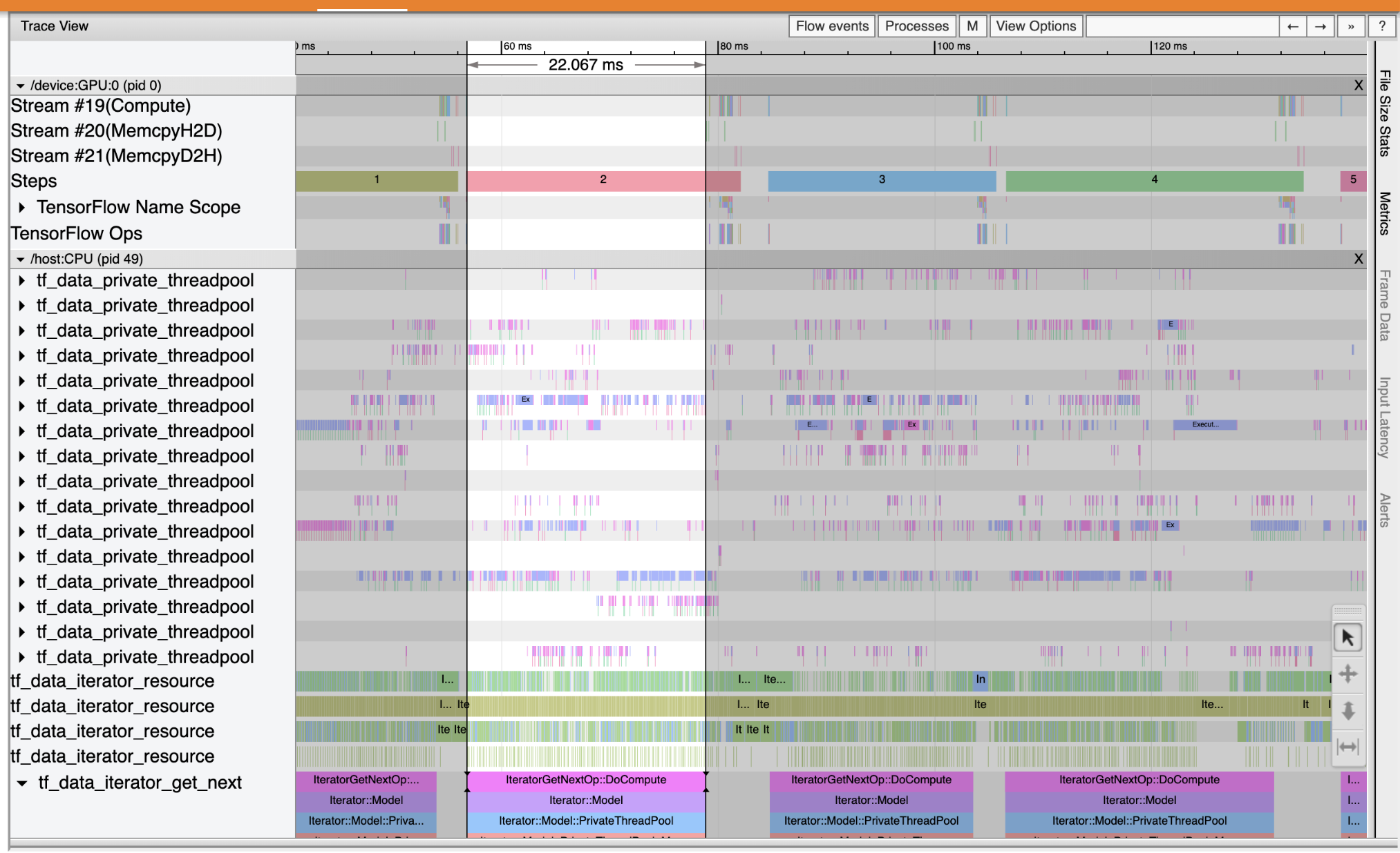
Looking at the event traces, you can see that the GPU is inactive while the tf_data_iterator_get_next op is running on the CPU. This op is responsible for processing the input data and sending it to the GPU for training. As a general rule of thumb, it is a good idea to always keep the device (GPU/TPU) active.
Use the tf.data API to optimize the input pipeline. In this case, let's cache the training dataset and prefetch the data to ensure that there is always data available for the GPU to process. See here for more details on using tf.data to optimize your input pipelines.
(ds_train, ds_test), ds_info = tfds.load(
    'mnist',
    split=['train', 'test'],
    shuffle_files=True,
    as_supervised=True,
    with_info=True,
)
ds_train = ds_train.map(normalize_img)
ds_train = ds_train.batch(128)
ds_train = ds_train.cache()
ds_train = ds_train.prefetch(tf.data.experimental.AUTOTUNE)
ds_test = ds_test.map(normalize_img)
ds_test = ds_test.batch(128)
ds_test = ds_test.cache()
ds_test = ds_test.prefetch(tf.data.experimental.AUTOTUNE)
Train the model again and capture the performance profile by reusing the callback from before.
model.fit(ds_train,
          epochs=2,
          validation_data=ds_test,
          callbacks = [tboard_callback])
Epoch 1/2
469/469 [==============================] - 10s 22ms/step - loss: 0.1194 - accuracy: 0.9658 - val_loss: 0.1116 - val_accuracy: 0.9680
Epoch 2/2
469/469 [==============================] - 1s 3ms/step - loss: 0.0918 - accuracy: 0.9740 - val_loss: 0.0979 - val_accuracy: 0.9712
<tensorflow.python.keras.callbacks.History at 0x7f23908762b0>
Re-launch TensorBoard and open the Profile tab to observe the performance profile for the updated input pipeline.
The performance profile for the model with the optimized input pipeline is similar to the image below.
%tensorboard --logdir=logs
Reusing TensorBoard on port 6006 (pid 750), started 0:00:12 ago. (Use '!kill 750' to kill it.)
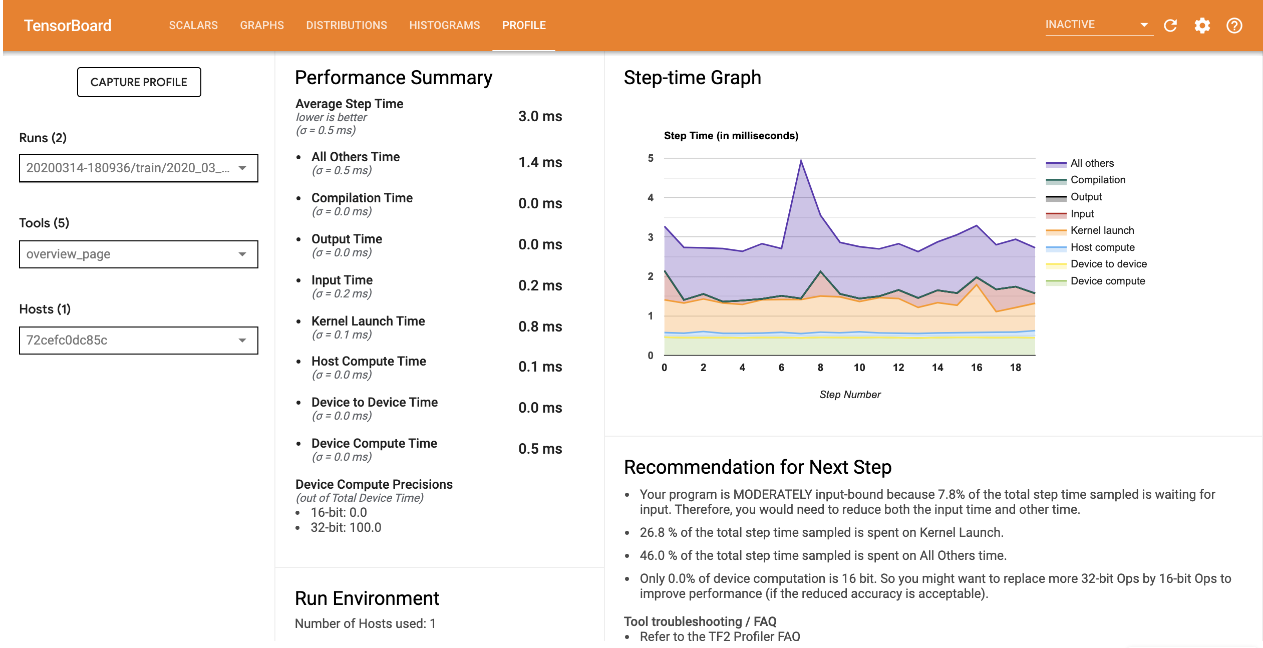
From the Overview page, you can see that the Average Step time has reduced as has the Input Step time. The Step-time Graph also indicates that the model is no longer highly input bound. Open the Trace Viewer to examine the trace events with the optimized input pipeline.
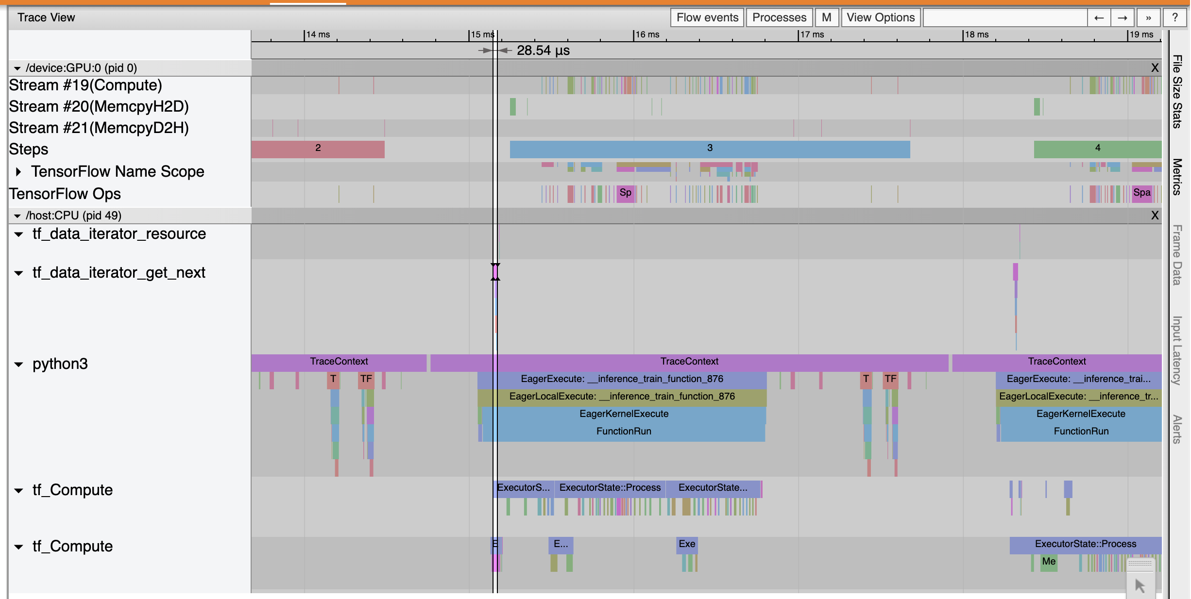
The Trace Viewer shows that the tf_data_iterator_get_next op executes much faster. The GPU therefore gets a steady stream of data to perform training and achieves much better utilization through model training.
Summary
Use the TensorFlow Profiler to profile and debug model training performance. Read the Profiler guide and watch the Performance profiling in TF 2 talk from the TensorFlow Dev Summit 2020 to learn more about the TensorFlow Profiler.