Handwritten digits recognition (using Multilayer Perceptron)
- 🤖 See full list of Machine Learning Experiments on GitHub
- ▶️ Interactive Demo: try this model and other machine learning experiments in action
Experiment overview
In this experiment we will build a Multilayer Perceptron (MLP) model using Tensorflow to recognize handwritten digits.
A multilayer perceptron (MLP) is a class of feedforward artificial neural network. An MLP consists of, at least, three layers of nodes: an input layer, a hidden layer and an output layer. Except for the input nodes, each node is a neuron that uses a nonlinear activation function. MLP utilizes a supervised learning technique called backpropagation for training. Its multiple layers and non-linear activation distinguish MLP from a linear perceptron. It can distinguish data that is not linearly separable.
Import dependencies
- tensorflow - for developing and training ML models.
- matplotlib - for plotting the data.
- seaborn - for plotting confusion matrix.
- numpy - for linear algebra operations.
- pandas - for displaying training/test data in a table.
- math - for calculating square roots etc.
- datetime - for generating a logs folder names.
# Selecting Tensorflow version v2 (the command is relevant for Colab only).
%tensorflow_version 2.x
import tensorflow as tf
import matplotlib.pyplot as plt
import seaborn as sn
import numpy as np
import pandas as pd
import math
import datetime
import platform

print('Python version:', platform.python_version())
print('Tensorflow version:', tf.__version__)
print('Keras version:', tf.keras.__version__)
Python version: 3.7.6
Tensorflow version: 2.1.0
Keras version: 2.2.4-tf
Configuring Tensorboard
We will use Tensorboard to debug the model later.
# Load the TensorBoard notebook extension.
# %reload_ext tensorboard
%load_ext tensorboard
# Clear any logs from previous runs.
!rm -rf ./.logs/
Load the data
The training dataset consists of 60000 28x28px images of hand-written digits from 0 to 9.
The test dataset consists of 10000 28x28px images.
mnist_dataset = tf.keras.datasets.mnist
(x_train, y_train), (x_test, y_test) = mnist_dataset.load_data()
print('x_train:', x_train.shape)
print('y_train:', y_train.shape)
print('x_test:', x_test.shape)
print('y_test:', y_test.shape)
x_train: (60000, 28, 28)
y_train: (60000,)
x_test: (10000, 28, 28)
y_test: (10000,)
Explore the data
Here is how each image in the dataset looks like. It is a 28x28 matrix of integers (from 0 to 255). Each integer represents a color of a pixel.
pd.DataFrame(x_train[0])
| 0 | 1 | 2 | 3 | 4 | 5 | 6 | 7 | 8 | 9 | ... | 18 | 19 | 20 | 21 | 22 | 23 | 24 | 25 | 26 | 27 | |
|---|---|---|---|---|---|---|---|---|---|---|---|---|---|---|---|---|---|---|---|---|---|
| 0 | 0 | 0 | 0 | 0 | 0 | 0 | 0 | 0 | 0 | 0 | ... | 0 | 0 | 0 | 0 | 0 | 0 | 0 | 0 | 0 | 0 |
| 1 | 0 | 0 | 0 | 0 | 0 | 0 | 0 | 0 | 0 | 0 | ... | 0 | 0 | 0 | 0 | 0 | 0 | 0 | 0 | 0 | 0 |
| 2 | 0 | 0 | 0 | 0 | 0 | 0 | 0 | 0 | 0 | 0 | ... | 0 | 0 | 0 | 0 | 0 | 0 | 0 | 0 | 0 | 0 |
| 3 | 0 | 0 | 0 | 0 | 0 | 0 | 0 | 0 | 0 | 0 | ... | 0 | 0 | 0 | 0 | 0 | 0 | 0 | 0 | 0 | 0 |
| 4 | 0 | 0 | 0 | 0 | 0 | 0 | 0 | 0 | 0 | 0 | ... | 0 | 0 | 0 | 0 | 0 | 0 | 0 | 0 | 0 | 0 |
| 5 | 0 | 0 | 0 | 0 | 0 | 0 | 0 | 0 | 0 | 0 | ... | 175 | 26 | 166 | 255 | 247 | 127 | 0 | 0 | 0 | 0 |
| 6 | 0 | 0 | 0 | 0 | 0 | 0 | 0 | 0 | 30 | 36 | ... | 225 | 172 | 253 | 242 | 195 | 64 | 0 | 0 | 0 | 0 |
| 7 | 0 | 0 | 0 | 0 | 0 | 0 | 0 | 49 | 238 | 253 | ... | 93 | 82 | 82 | 56 | 39 | 0 | 0 | 0 | 0 | 0 |
| 8 | 0 | 0 | 0 | 0 | 0 | 0 | 0 | 18 | 219 | 253 | ... | 0 | 0 | 0 | 0 | 0 | 0 | 0 | 0 | 0 | 0 |
| 9 | 0 | 0 | 0 | 0 | 0 | 0 | 0 | 0 | 80 | 156 | ... | 0 | 0 | 0 | 0 | 0 | 0 | 0 | 0 | 0 | 0 |
| 10 | 0 | 0 | 0 | 0 | 0 | 0 | 0 | 0 | 0 | 14 | ... | 0 | 0 | 0 | 0 | 0 | 0 | 0 | 0 | 0 | 0 |
| 11 | 0 | 0 | 0 | 0 | 0 | 0 | 0 | 0 | 0 | 0 | ... | 0 | 0 | 0 | 0 | 0 | 0 | 0 | 0 | 0 | 0 |
| 12 | 0 | 0 | 0 | 0 | 0 | 0 | 0 | 0 | 0 | 0 | ... | 0 | 0 | 0 | 0 | 0 | 0 | 0 | 0 | 0 | 0 |
| 13 | 0 | 0 | 0 | 0 | 0 | 0 | 0 | 0 | 0 | 0 | ... | 0 | 0 | 0 | 0 | 0 | 0 | 0 | 0 | 0 | 0 |
| 14 | 0 | 0 | 0 | 0 | 0 | 0 | 0 | 0 | 0 | 0 | ... | 25 | 0 | 0 | 0 | 0 | 0 | 0 | 0 | 0 | 0 |
| 15 | 0 | 0 | 0 | 0 | 0 | 0 | 0 | 0 | 0 | 0 | ... | 150 | 27 | 0 | 0 | 0 | 0 | 0 | 0 | 0 | 0 |
| 16 | 0 | 0 | 0 | 0 | 0 | 0 | 0 | 0 | 0 | 0 | ... | 253 | 187 | 0 | 0 | 0 | 0 | 0 | 0 | 0 | 0 |
| 17 | 0 | 0 | 0 | 0 | 0 | 0 | 0 | 0 | 0 | 0 | ... | 253 | 249 | 64 | 0 | 0 | 0 | 0 | 0 | 0 | 0 |
| 18 | 0 | 0 | 0 | 0 | 0 | 0 | 0 | 0 | 0 | 0 | ... | 253 | 207 | 2 | 0 | 0 | 0 | 0 | 0 | 0 | 0 |
| 19 | 0 | 0 | 0 | 0 | 0 | 0 | 0 | 0 | 0 | 0 | ... | 250 | 182 | 0 | 0 | 0 | 0 | 0 | 0 | 0 | 0 |
| 20 | 0 | 0 | 0 | 0 | 0 | 0 | 0 | 0 | 0 | 0 | ... | 78 | 0 | 0 | 0 | 0 | 0 | 0 | 0 | 0 | 0 |
| 21 | 0 | 0 | 0 | 0 | 0 | 0 | 0 | 0 | 23 | 66 | ... | 0 | 0 | 0 | 0 | 0 | 0 | 0 | 0 | 0 | 0 |
| 22 | 0 | 0 | 0 | 0 | 0 | 0 | 18 | 171 | 219 | 253 | ... | 0 | 0 | 0 | 0 | 0 | 0 | 0 | 0 | 0 | 0 |
| 23 | 0 | 0 | 0 | 0 | 55 | 172 | 226 | 253 | 253 | 253 | ... | 0 | 0 | 0 | 0 | 0 | 0 | 0 | 0 | 0 | 0 |
| 24 | 0 | 0 | 0 | 0 | 136 | 253 | 253 | 253 | 212 | 135 | ... | 0 | 0 | 0 | 0 | 0 | 0 | 0 | 0 | 0 | 0 |
| 25 | 0 | 0 | 0 | 0 | 0 | 0 | 0 | 0 | 0 | 0 | ... | 0 | 0 | 0 | 0 | 0 | 0 | 0 | 0 | 0 | 0 |
| 26 | 0 | 0 | 0 | 0 | 0 | 0 | 0 | 0 | 0 | 0 | ... | 0 | 0 | 0 | 0 | 0 | 0 | 0 | 0 | 0 | 0 |
| 27 | 0 | 0 | 0 | 0 | 0 | 0 | 0 | 0 | 0 | 0 | ... | 0 | 0 | 0 | 0 | 0 | 0 | 0 | 0 | 0 | 0 |
28 rows × 28 columns
This matrix of numbers may be drawn as follows:
plt.imshow(x_train[0], cmap=plt.cm.binary)
plt.show()

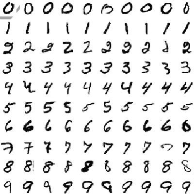
Let's print some more training examples to get the feeling of how the digits were written.
numbers_to_display = 25
num_cells = math.ceil(math.sqrt(numbers_to_display))
plt.figure(figsize=(10,10))
for i in range(numbers_to_display):
    plt.subplot(num_cells, num_cells, i+1)
    plt.xticks([])
    plt.yticks([])
    plt.grid(False)
    plt.imshow(x_train[i], cmap=plt.cm.binary)
    plt.xlabel(y_train[i])
plt.show()

Normalize the data
Here we're just trying to move from values range of [0...255] to [0...1].
x_train_normalized = x_train / 255
x_test_normalized = x_test / 255
with pd.option_context('display.float_format', '{:,.2f}'.format):
    display(pd.DataFrame(x_train_normalized[0]))
| 0 | 1 | 2 | 3 | 4 | 5 | 6 | 7 | 8 | 9 | ... | 18 | 19 | 20 | 21 | 22 | 23 | 24 | 25 | 26 | 27 | |
|---|---|---|---|---|---|---|---|---|---|---|---|---|---|---|---|---|---|---|---|---|---|
| 0 | 0.00 | 0.00 | 0.00 | 0.00 | 0.00 | 0.00 | 0.00 | 0.00 | 0.00 | 0.00 | ... | 0.00 | 0.00 | 0.00 | 0.00 | 0.00 | 0.00 | 0.00 | 0.00 | 0.00 | 0.00 |
| 1 | 0.00 | 0.00 | 0.00 | 0.00 | 0.00 | 0.00 | 0.00 | 0.00 | 0.00 | 0.00 | ... | 0.00 | 0.00 | 0.00 | 0.00 | 0.00 | 0.00 | 0.00 | 0.00 | 0.00 | 0.00 |
| 2 | 0.00 | 0.00 | 0.00 | 0.00 | 0.00 | 0.00 | 0.00 | 0.00 | 0.00 | 0.00 | ... | 0.00 | 0.00 | 0.00 | 0.00 | 0.00 | 0.00 | 0.00 | 0.00 | 0.00 | 0.00 |
| 3 | 0.00 | 0.00 | 0.00 | 0.00 | 0.00 | 0.00 | 0.00 | 0.00 | 0.00 | 0.00 | ... | 0.00 | 0.00 | 0.00 | 0.00 | 0.00 | 0.00 | 0.00 | 0.00 | 0.00 | 0.00 |
| 4 | 0.00 | 0.00 | 0.00 | 0.00 | 0.00 | 0.00 | 0.00 | 0.00 | 0.00 | 0.00 | ... | 0.00 | 0.00 | 0.00 | 0.00 | 0.00 | 0.00 | 0.00 | 0.00 | 0.00 | 0.00 |
| 5 | 0.00 | 0.00 | 0.00 | 0.00 | 0.00 | 0.00 | 0.00 | 0.00 | 0.00 | 0.00 | ... | 0.69 | 0.10 | 0.65 | 1.00 | 0.97 | 0.50 | 0.00 | 0.00 | 0.00 | 0.00 |
| 6 | 0.00 | 0.00 | 0.00 | 0.00 | 0.00 | 0.00 | 0.00 | 0.00 | 0.12 | 0.14 | ... | 0.88 | 0.67 | 0.99 | 0.95 | 0.76 | 0.25 | 0.00 | 0.00 | 0.00 | 0.00 |
| 7 | 0.00 | 0.00 | 0.00 | 0.00 | 0.00 | 0.00 | 0.00 | 0.19 | 0.93 | 0.99 | ... | 0.36 | 0.32 | 0.32 | 0.22 | 0.15 | 0.00 | 0.00 | 0.00 | 0.00 | 0.00 |
| 8 | 0.00 | 0.00 | 0.00 | 0.00 | 0.00 | 0.00 | 0.00 | 0.07 | 0.86 | 0.99 | ... | 0.00 | 0.00 | 0.00 | 0.00 | 0.00 | 0.00 | 0.00 | 0.00 | 0.00 | 0.00 |
| 9 | 0.00 | 0.00 | 0.00 | 0.00 | 0.00 | 0.00 | 0.00 | 0.00 | 0.31 | 0.61 | ... | 0.00 | 0.00 | 0.00 | 0.00 | 0.00 | 0.00 | 0.00 | 0.00 | 0.00 | 0.00 |
| 10 | 0.00 | 0.00 | 0.00 | 0.00 | 0.00 | 0.00 | 0.00 | 0.00 | 0.00 | 0.05 | ... | 0.00 | 0.00 | 0.00 | 0.00 | 0.00 | 0.00 | 0.00 | 0.00 | 0.00 | 0.00 |
| 11 | 0.00 | 0.00 | 0.00 | 0.00 | 0.00 | 0.00 | 0.00 | 0.00 | 0.00 | 0.00 | ... | 0.00 | 0.00 | 0.00 | 0.00 | 0.00 | 0.00 | 0.00 | 0.00 | 0.00 | 0.00 |
| 12 | 0.00 | 0.00 | 0.00 | 0.00 | 0.00 | 0.00 | 0.00 | 0.00 | 0.00 | 0.00 | ... | 0.00 | 0.00 | 0.00 | 0.00 | 0.00 | 0.00 | 0.00 | 0.00 | 0.00 | 0.00 |
| 13 | 0.00 | 0.00 | 0.00 | 0.00 | 0.00 | 0.00 | 0.00 | 0.00 | 0.00 | 0.00 | ... | 0.00 | 0.00 | 0.00 | 0.00 | 0.00 | 0.00 | 0.00 | 0.00 | 0.00 | 0.00 |
| 14 | 0.00 | 0.00 | 0.00 | 0.00 | 0.00 | 0.00 | 0.00 | 0.00 | 0.00 | 0.00 | ... | 0.10 | 0.00 | 0.00 | 0.00 | 0.00 | 0.00 | 0.00 | 0.00 | 0.00 | 0.00 |
| 15 | 0.00 | 0.00 | 0.00 | 0.00 | 0.00 | 0.00 | 0.00 | 0.00 | 0.00 | 0.00 | ... | 0.59 | 0.11 | 0.00 | 0.00 | 0.00 | 0.00 | 0.00 | 0.00 | 0.00 | 0.00 |
| 16 | 0.00 | 0.00 | 0.00 | 0.00 | 0.00 | 0.00 | 0.00 | 0.00 | 0.00 | 0.00 | ... | 0.99 | 0.73 | 0.00 | 0.00 | 0.00 | 0.00 | 0.00 | 0.00 | 0.00 | 0.00 |
| 17 | 0.00 | 0.00 | 0.00 | 0.00 | 0.00 | 0.00 | 0.00 | 0.00 | 0.00 | 0.00 | ... | 0.99 | 0.98 | 0.25 | 0.00 | 0.00 | 0.00 | 0.00 | 0.00 | 0.00 | 0.00 |
| 18 | 0.00 | 0.00 | 0.00 | 0.00 | 0.00 | 0.00 | 0.00 | 0.00 | 0.00 | 0.00 | ... | 0.99 | 0.81 | 0.01 | 0.00 | 0.00 | 0.00 | 0.00 | 0.00 | 0.00 | 0.00 |
| 19 | 0.00 | 0.00 | 0.00 | 0.00 | 0.00 | 0.00 | 0.00 | 0.00 | 0.00 | 0.00 | ... | 0.98 | 0.71 | 0.00 | 0.00 | 0.00 | 0.00 | 0.00 | 0.00 | 0.00 | 0.00 |
| 20 | 0.00 | 0.00 | 0.00 | 0.00 | 0.00 | 0.00 | 0.00 | 0.00 | 0.00 | 0.00 | ... | 0.31 | 0.00 | 0.00 | 0.00 | 0.00 | 0.00 | 0.00 | 0.00 | 0.00 | 0.00 |
| 21 | 0.00 | 0.00 | 0.00 | 0.00 | 0.00 | 0.00 | 0.00 | 0.00 | 0.09 | 0.26 | ... | 0.00 | 0.00 | 0.00 | 0.00 | 0.00 | 0.00 | 0.00 | 0.00 | 0.00 | 0.00 |
| 22 | 0.00 | 0.00 | 0.00 | 0.00 | 0.00 | 0.00 | 0.07 | 0.67 | 0.86 | 0.99 | ... | 0.00 | 0.00 | 0.00 | 0.00 | 0.00 | 0.00 | 0.00 | 0.00 | 0.00 | 0.00 |
| 23 | 0.00 | 0.00 | 0.00 | 0.00 | 0.22 | 0.67 | 0.89 | 0.99 | 0.99 | 0.99 | ... | 0.00 | 0.00 | 0.00 | 0.00 | 0.00 | 0.00 | 0.00 | 0.00 | 0.00 | 0.00 |
| 24 | 0.00 | 0.00 | 0.00 | 0.00 | 0.53 | 0.99 | 0.99 | 0.99 | 0.83 | 0.53 | ... | 0.00 | 0.00 | 0.00 | 0.00 | 0.00 | 0.00 | 0.00 | 0.00 | 0.00 | 0.00 |
| 25 | 0.00 | 0.00 | 0.00 | 0.00 | 0.00 | 0.00 | 0.00 | 0.00 | 0.00 | 0.00 | ... | 0.00 | 0.00 | 0.00 | 0.00 | 0.00 | 0.00 | 0.00 | 0.00 | 0.00 | 0.00 |
| 26 | 0.00 | 0.00 | 0.00 | 0.00 | 0.00 | 0.00 | 0.00 | 0.00 | 0.00 | 0.00 | ... | 0.00 | 0.00 | 0.00 | 0.00 | 0.00 | 0.00 | 0.00 | 0.00 | 0.00 | 0.00 |
| 27 | 0.00 | 0.00 | 0.00 | 0.00 | 0.00 | 0.00 | 0.00 | 0.00 | 0.00 | 0.00 | ... | 0.00 | 0.00 | 0.00 | 0.00 | 0.00 | 0.00 | 0.00 | 0.00 | 0.00 | 0.00 |
28 rows × 28 columns
Let's see how the digits look like after normalization. We're expecting it to look similar to original.
plt.imshow(x_train_normalized[0], cmap=plt.cm.binary)
plt.show()
Build the model
We will use Sequential Keras model with 4 layers:
- Layer 1: Flatten layer that will flatten image 2D matrix into 1D vector.
- Layer 2: Input Dense layer with
128neurons and ReLU activation. - Layer 3: Hidden Dense layer with
128neurons and ReLU activation. - Layer 4: Output Dense layer with
10Softmax outputs. The output represents the network guess. The 0-th output represents a probability that the input digit is0, the 1-st output represents a probability that the input digit is1and so on...
In this example we will use kernel_regularizer parameter of the layer to control overfitting of the model. Another common approach to fight overfitting though might be using a dropout layers (i.e. tf.keras.layers.Dropout(0.2)).
model = tf.keras.models.Sequential()

# Input layers.
model.add(tf.keras.layers.Flatten(input_shape=x_train_normalized.shape[1:]))
model.add(tf.keras.layers.Dense(
    units=128,
    activation=tf.keras.activations.relu,
    kernel_regularizer=tf.keras.regularizers.l2(0.002)
))

# Hidden layers.
model.add(tf.keras.layers.Dense(
    units=128,
    activation=tf.keras.activations.relu,
    kernel_regularizer=tf.keras.regularizers.l2(0.002)
))

# Output layers.
model.add(tf.keras.layers.Dense(
    units=10,
    activation=tf.keras.activations.softmax
))
Here is our model summary so far.
model.summary()
Model: "sequential"
_________________________________________________________________
Layer (type)                 Output Shape              Param #
=================================================================
flatten (Flatten)            (None, 784)               0
_________________________________________________________________
dense (Dense)                (None, 128)               100480
_________________________________________________________________
dense_1 (Dense)              (None, 128)               16512
_________________________________________________________________
dense_2 (Dense)              (None, 10)                1290
=================================================================
Total params: 118,282
Trainable params: 118,282
Non-trainable params: 0
_________________________________________________________________
In order to plot the model the graphviz should be installed. For Mac OS it may be installed using brew like brew install graphviz.
tf.keras.utils.plot_model(
    model,
    show_shapes=True,
    show_layer_names=True,
)

Compile the model
adam_optimizer = tf.keras.optimizers.Adam(learning_rate=0.001)

model.compile(
    optimizer=adam_optimizer,
    loss=tf.keras.losses.sparse_categorical_crossentropy,
    metrics=['accuracy']
)
Train the model
log_dir=".logs/fit/" + datetime.datetime.now().strftime("%Y%m%d-%H%M%S")
tensorboard_callback = tf.keras.callbacks.TensorBoard(log_dir=log_dir, histogram_freq=1)

training_history = model.fit(
    x_train_normalized,
    y_train,
    epochs=10,
    validation_data=(x_test_normalized, y_test),
    callbacks=[tensorboard_callback]
)
Train on 60000 samples, validate on 10000 samples
Epoch 1/10
60000/60000 [==============================] - 10s 173us/sample - loss: 0.5159 - accuracy: 0.9247 - val_loss: 0.3251 - val_accuracy: 0.9512
Epoch 2/10
60000/60000 [==============================] - 12s 195us/sample - loss: 0.2996 - accuracy: 0.9546 - val_loss: 0.2767 - val_accuracy: 0.9558
Epoch 3/10
60000/60000 [==============================] - 11s 180us/sample - loss: 0.2624 - accuracy: 0.9600 - val_loss: 0.2342 - val_accuracy: 0.9675
Epoch 4/10
60000/60000 [==============================] - 10s 174us/sample - loss: 0.2408 - accuracy: 0.9629 - val_loss: 0.2276 - val_accuracy: 0.9650
Epoch 5/10
60000/60000 [==============================] - 8s 138us/sample - loss: 0.2257 - accuracy: 0.9645 - val_loss: 0.2415 - val_accuracy: 0.9584
Epoch 6/10
60000/60000 [==============================] - 8s 139us/sample - loss: 0.2148 - accuracy: 0.9669 - val_loss: 0.2188 - val_accuracy: 0.9639
Epoch 7/10
60000/60000 [==============================] - 10s 164us/sample - loss: 0.2044 - accuracy: 0.9689 - val_loss: 0.1923 - val_accuracy: 0.9707
Epoch 8/10
60000/60000 [==============================] - 8s 139us/sample - loss: 0.1980 - accuracy: 0.9688 - val_loss: 0.2008 - val_accuracy: 0.9662
Epoch 9/10
60000/60000 [==============================] - 9s 146us/sample - loss: 0.1940 - accuracy: 0.9685 - val_loss: 0.2088 - val_accuracy: 0.9641
Epoch 10/10
60000/60000 [==============================] - 7s 116us/sample - loss: 0.1906 - accuracy: 0.9693 - val_loss: 0.2004 - val_accuracy: 0.9646
Let's see how the loss function was changing during the training. We expect it to get smaller and smaller on every next epoch.
plt.xlabel('Epoch Number')
plt.ylabel('Loss')
plt.plot(training_history.history['loss'], label='training set')
plt.plot(training_history.history['val_loss'], label='test set')
plt.legend()
<matplotlib.legend.Legend at 0x1406d4750>

plt.xlabel('Epoch Number')
plt.ylabel('Accuracy')
plt.plot(training_history.history['accuracy'], label='training set')
plt.plot(training_history.history['val_accuracy'], label='test set')
plt.legend()
<matplotlib.legend.Legend at 0x14069cbd0>

Evaluate model accuracy
We need to compare the accuracy of our model on training set and on test set. We expect our model to perform similarly on both sets. If the performance on a test set will be poor comparing to a training set it would be an indicator for us that the model is overfitted and we have a "high variance" issue.
Training set accuracy
%%capture
train_loss, train_accuracy = model.evaluate(x_train_normalized, y_train)
print('Training loss: ', train_loss)
print('Training accuracy: ', train_accuracy)
Training loss:  0.1835839938680331
Training accuracy:  0.97095
Test set accuracy
%%capture
validation_loss, validation_accuracy = model.evaluate(x_test_normalized, y_test)
print('Validation loss: ', validation_loss)
print('Validation accuracy: ', validation_accuracy)
Validation loss:  0.2004156953573227
Validation accuracy:  0.9646
Save the model
We will save the entire model to a HDF5 file. The .h5 extension of the file indicates that the model should be saved in Keras format as HDF5 file. To use this model on the front-end we will convert it (later in this notebook) to Javascript understandable format (tfjs_layers_model with .json and .bin files) using tensorflowjs_converter as it is specified in the main README.
model_name = 'digits_recognition_mlp.h5'
model.save(model_name, save_format='h5')
loaded_model = tf.keras.models.load_model(model_name)
Use the model (do predictions)
To use the model that we've just trained for digits recognition we need to call predict() method.
predictions_one_hot = loaded_model.predict([x_test_normalized])
print('predictions_one_hot:', predictions_one_hot.shape)
predictions_one_hot: (10000, 10)
Each prediction consists of 10 probabilities (one for each number from 0 to 9). We need to pick the digit with the highest probability since this would be a digit that our model most confident with.
# Predictions in form of one-hot vectors (arrays of probabilities).
pd.DataFrame(predictions_one_hot)
| 0 | 1 | 2 | 3 | 4 | 5 | 6 | 7 | 8 | 9 | |
|---|---|---|---|---|---|---|---|---|---|---|
| 0 | 7.774682e-07 | 1.361266e-05 | 9.182121e-05 | 1.480533e-04 | 3.271606e-08 | 2.764984e-06 | 5.903113e-11 | 9.996371e-01 | 1.666906e-06 | 1.042360e-04 |
| 1 | 1.198126e-03 | 1.047034e-04 | 9.888538e-01 | 3.167473e-03 | 2.532723e-08 | 8.854911e-04 | 6.828848e-04 | 5.048555e-06 | 5.102141e-03 | 2.777219e-07 |
| 2 | 8.876222e-07 | 9.985157e-01 | 7.702865e-05 | 2.815677e-05 | 5.406159e-04 | 2.707353e-05 | 2.035172e-04 | 9.576474e-05 | 5.053744e-04 | 5.977653e-06 |
| 3 | 9.990014e-01 | 4.625264e-06 | 5.582303e-04 | 5.484722e-06 | 3.299095e-05 | 2.761683e-05 | 1.418936e-04 | 1.374896e-04 | 1.264711e-06 | 8.899846e-05 |
| 4 | 1.575061e-04 | 3.707617e-06 | 9.205778e-06 | 3.638557e-07 | 9.973990e-01 | 1.538193e-06 | 3.079933e-05 | 4.155232e-05 | 4.639028e-06 | 2.351647e-03 |
| ... | ... | ... | ... | ... | ... | ... | ... | ... | ... | ... |
| 9995 | 1.657425e-07 | 8.666945e-04 | 9.987835e-01 | 2.244577e-04 | 6.904386e-12 | 1.850143e-07 | 4.015289e-08 | 9.534077e-05 | 2.960863e-05 | 4.335253e-10 |
| 9996 | 6.585806e-09 | 6.717554e-06 | 6.165197e-06 | 9.982822e-01 | 2.519031e-09 | 1.577783e-03 | 5.583775e-11 | 2.066899e-06 | 1.257137e-05 | 1.125286e-04 |
| 9997 | 3.056851e-08 | 6.843247e-06 | 3.161353e-09 | 6.484316e-08 | 9.989114e-01 | 2.373860e-07 | 1.930965e-08 | 1.753431e-05 | 5.452521e-06 | 1.058474e-03 |
| 9998 | 7.249156e-06 | 5.103301e-07 | 2.712475e-08 | 1.025373e-04 | 5.019490e-08 | 9.996431e-01 | 9.364716e-05 | 1.444746e-07 | 1.520906e-04 | 6.703385e-07 |
| 9999 | 2.355737e-06 | 4.141651e-07 | 4.489176e-06 | 1.321389e-07 | 2.956528e-05 | 3.940167e-05 | 9.999231e-01 | 7.314535e-08 | 2.270459e-07 | 1.044889e-07 |
10000 rows × 10 columns
# Let's extract predictions with highest probabilites and detect what digits have been actually recognized.
predictions = np.argmax(predictions_one_hot, axis=1)
pd.DataFrame(predictions)
| 0 | |
|---|---|
| 0 | 7 |
| 1 | 2 |
| 2 | 1 |
| 3 | 0 |
| 4 | 4 |
| ... | ... |
| 9995 | 2 |
| 9996 | 3 |
| 9997 | 4 |
| 9998 | 5 |
| 9999 | 6 |
10000 rows × 1 columns
So our model is predicting that the first example from the test set is 7.
print(predictions[0])
7
Let's print the first image from a test set to see if model's prediction is correct.
plt.imshow(x_test_normalized[0], cmap=plt.cm.binary)
plt.show()

We see that our model made a correct prediction and it successfully recognized digit 7. Let's print some more test examples and correspondent predictions to see how model performs and where it does mistakes.
numbers_to_display = 196
num_cells = math.ceil(math.sqrt(numbers_to_display))
plt.figure(figsize=(15, 15))

for plot_index in range(numbers_to_display):
    predicted_label = predictions[plot_index]
    plt.xticks([])
    plt.yticks([])
    plt.grid(False)
    color_map = 'Greens' if predicted_label == y_test[plot_index] else 'Reds'
    plt.subplot(num_cells, num_cells, plot_index + 1)
    plt.imshow(x_test_normalized[plot_index], cmap=color_map)
    plt.xlabel(predicted_label)

plt.subplots_adjust(hspace=1, wspace=0.5)
plt.show()

Plotting a confusion matrix
Confusion matrix shows what numbers are recognized well by the model and what numbers the model usually confuses to recognize correctly. You may see that the model performs really well but sometimes (28 times out of 10000) it may confuse number 5 with 3 or number 2 with 3.
confusion_matrix = tf.math.confusion_matrix(y_test, predictions)
f, ax = plt.subplots(figsize=(9, 7))
sn.heatmap(
    confusion_matrix,
    annot=True,
    linewidths=.5,
    fmt="d",
    square=True,
    ax=ax
)
plt.show()

Debugging the model with TensorBoard
TensorBoard is a tool for providing the measurements and visualizations needed during the machine learning workflow. It enables tracking experiment metrics like loss and accuracy, visualizing the model graph, projecting embeddings to a lower dimensional space, and much more.
%tensorboard --logdir .logs/fit
/bin/sh: line 0: kill: (43638) - No such process
Converting the model to web-format
To use this model on the web we need to convert it into the format that will be understandable by tensorflowjs. To do so we may use tfjs-converter as following:
tensorflowjs_converter --input_format keras \
  ./experiments/digits_recognition_mlp/digits_recognition_mlp.h5 \
  ./demos/public/models/digits_recognition_mlp
You find this experiment in the Demo app and play around with it right in you browser to see how the model performs in real life.