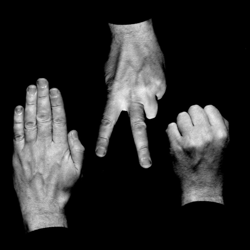
Rock Paper Scissors (using Convolutional Neural Network)
- 🤖 See full list of Machine Learning Experiments on GitHub
- ▶️ Interactive Demo: try this model and other machine learning experiments in action
Experiment overview
In this experiment we will build a Convolutional Neural Network (CNN) model using Tensorflow to recognize Rock-Paper-Scissors signs (gestures) on the photo.
A convolutional neural network (CNN, or ConvNet) is a Deep Learning algorithm which can take in an input image, assign importance (learnable weights and biases) to various aspects/objects in the image and be able to differentiate one from the other.
Inspired by Getting started with TensorFlow 2.0 article.
Importing dependencies
# Selecting Tensorflow version v2 (the command is relevant for Colab only).
%tensorflow_version 2.x
UsageError: Line magic function `%tensorflow_version` not found.
import tensorflow as tf
import tensorflow_datasets as tfds
import matplotlib.pyplot as plt
import numpy as np
import platform
import datetime
import os
import math
import random

print('Python version:', platform.python_version())
print('Tensorflow version:', tf.__version__)
print('Keras version:', tf.keras.__version__)
Python version: 3.6.9
Tensorflow version: 2.1.0
Keras version: 2.2.4-tf
Configuring TensorBoard
We will use TensorBoard as a helper to debug the model training process.
# Load the TensorBoard notebook extension.
# %reload_ext tensorboard
%load_ext tensorboard
# Clear any logs from previous runs.
!rm -rf ./logs/
Loading the dataset
We will download Rock-Paper-Scissors dataset from TensorFlow Datasets collection. To do that we loaded a tensorflow_datasets module.
tensorflow_datasets defines a collection of datasets ready-to-use with TensorFlow.
Each dataset is defined as a tfds.core.DatasetBuilder, which encapsulates the logic to download the dataset and construct an input pipeline, as well as contains the dataset documentation (version, splits, number of examples, etc.).
# See available datasets
tfds.list_builders()
['abstract_reasoning',
 'aeslc',
 'aflw2k3d',
 'amazon_us_reviews',
 'arc',
 'bair_robot_pushing_small',
 'big_patent',
 'bigearthnet',
 'billsum',
 'binarized_mnist',
 'binary_alpha_digits',
 'c4',
 'caltech101',
 'caltech_birds2010',
 'caltech_birds2011',
 'cars196',
 'cassava',
 'cats_vs_dogs',
 'celeb_a',
 'celeb_a_hq',
 'chexpert',
 'cifar10',
 'cifar100',
 'cifar10_1',
 'cifar10_corrupted',
 'citrus_leaves',
 'cityscapes',
 'civil_comments',
 'clevr',
 'cmaterdb',
 'cnn_dailymail',
 'coco',
 'coil100',
 'colorectal_histology',
 'colorectal_histology_large',
 'cos_e',
 'curated_breast_imaging_ddsm',
 'cycle_gan',
 'deep_weeds',
 'definite_pronoun_resolution',
 'diabetic_retinopathy_detection',
 'dmlab',
 'downsampled_imagenet',
 'dsprites',
 'dtd',
 'duke_ultrasound',
 'dummy_dataset_shared_generator',
 'dummy_mnist',
 'emnist',
 'esnli',
 'eurosat',
 'fashion_mnist',
 'flic',
 'flores',
 'food101',
 'gap',
 'gigaword',
 'glue',
 'groove',
 'higgs',
 'horses_or_humans',
 'i_naturalist2017',
 'image_label_folder',
 'imagenet2012',
 'imagenet2012_corrupted',
 'imagenet_resized',
 'imagenette',
 'imdb_reviews',
 'iris',
 'kitti',
 'kmnist',
 'lfw',
 'lm1b',
 'lost_and_found',
 'lsun',
 'malaria',
 'math_dataset',
 'mnist',
 'mnist_corrupted',
 'movie_rationales',
 'moving_mnist',
 'multi_news',
 'multi_nli',
 'multi_nli_mismatch',
 'newsroom',
 'nsynth',
 'omniglot',
 'open_images_v4',
 'oxford_flowers102',
 'oxford_iiit_pet',
 'para_crawl',
 'patch_camelyon',
 'pet_finder',
 'places365_small',
 'plant_leaves',
 'plant_village',
 'plantae_k',
 'quickdraw_bitmap',
 'reddit_tifu',
 'resisc45',
 'rock_paper_scissors',
 'rock_you',
 'scan',
 'scene_parse150',
 'scicite',
 'scientific_papers',
 'shapes3d',
 'smallnorb',
 'snli',
 'so2sat',
 'squad',
 'stanford_dogs',
 'stanford_online_products',
 'starcraft_video',
 'sun397',
 'super_glue',
 'svhn_cropped',
 'ted_hrlr_translate',
 'ted_multi_translate',
 'tf_flowers',
 'the300w_lp',
 'titanic',
 'trivia_qa',
 'uc_merced',
 'ucf101',
 'vgg_face2',
 'visual_domain_decathlon',
 'voc',
 'wider_face',
 'wikihow',
 'wikipedia',
 'wmt14_translate',
 'wmt15_translate',
 'wmt16_translate',
 'wmt17_translate',
 'wmt18_translate',
 'wmt19_translate',
 'wmt_t2t_translate',
 'wmt_translate',
 'xnli',
 'xsum']
DATASET_NAME = 'rock_paper_scissors'

(dataset_train_raw, dataset_test_raw), dataset_info = tfds.load(
    name=DATASET_NAME,
    data_dir='tmp',
    with_info=True,
    as_supervised=True,
    split=[tfds.Split.TRAIN, tfds.Split.TEST],
)
Downloading and preparing dataset rock_paper_scissors (219.53 MiB) to tmp/rock_paper_scissors/3.0.0...
HBox(children=(IntProgress(value=1, bar_style='info', description='Dl Completed...', max=1, style=ProgressStyl…
HBox(children=(IntProgress(value=1, bar_style='info', description='Dl Size...', max=1, style=ProgressStyle(des…
/usr/local/lib/python3.6/dist-packages/urllib3/connectionpool.py:847: InsecureRequestWarning: Unverified HTTPS request is being made. Adding certificate verification is strongly advised. See: https://urllib3.readthedocs.io/en/latest/advanced-usage.html#ssl-warnings
  InsecureRequestWarning)
/usr/local/lib/python3.6/dist-packages/urllib3/connectionpool.py:847: InsecureRequestWarning: Unverified HTTPS request is being made. Adding certificate verification is strongly advised. See: https://urllib3.readthedocs.io/en/latest/advanced-usage.html#ssl-warnings
  InsecureRequestWarning)
HBox(children=(IntProgress(value=1, bar_style='info', max=1), HTML(value='')))
Shuffling and writing examples to tmp/rock_paper_scissors/3.0.0.incompleteMDESME/rock_paper_scissors-train.tfrecord
HBox(children=(IntProgress(value=0, max=2520), HTML(value='')))
HBox(children=(IntProgress(value=1, bar_style='info', max=1), HTML(value='')))
Shuffling and writing examples to tmp/rock_paper_scissors/3.0.0.incompleteMDESME/rock_paper_scissors-test.tfrecord
HBox(children=(IntProgress(value=0, max=372), HTML(value='')))
Dataset rock_paper_scissors downloaded and prepared to tmp/rock_paper_scissors/3.0.0. Subsequent calls will reuse this data.
print('Raw train dataset:', dataset_train_raw)
print('Raw train dataset size:', len(list(dataset_train_raw)), '\n')

print('Raw test dataset:', dataset_test_raw)
print('Raw test dataset size:', len(list(dataset_test_raw)), '\n')
Raw train dataset: <DatasetV1Adapter shapes: ((300, 300, 3), ()), types: (tf.uint8, tf.int64)>
Raw train dataset size: 2520

Raw test dataset: <DatasetV1Adapter shapes: ((300, 300, 3), ()), types: (tf.uint8, tf.int64)>
Raw test dataset size: 372
dataset_info
tfds.core.DatasetInfo(
    name='rock_paper_scissors',
    version=3.0.0,
    description='Images of hands playing rock, paper, scissor game.',
    homepage='http://laurencemoroney.com/rock-paper-scissors-dataset',
    features=FeaturesDict({
        'image': Image(shape=(300, 300, 3), dtype=tf.uint8),
        'label': ClassLabel(shape=(), dtype=tf.int64, num_classes=3),
    }),
    total_num_examples=2892,
    splits={
        'test': 372,
        'train': 2520,
    },
    supervised_keys=('image', 'label'),
    citation="""@ONLINE {rps,
    author = "Laurence Moroney",
    title = "Rock, Paper, Scissors Dataset",
    month = "feb",
    year = "2019",
    url = "http://laurencemoroney.com/rock-paper-scissors-dataset"
    }""",
    redistribution_info=,
)
NUM_TRAIN_EXAMPLES = dataset_info.splits['train'].num_examples
NUM_TEST_EXAMPLES = dataset_info.splits['test'].num_examples
NUM_CLASSES = dataset_info.features['label'].num_classes

print('Number of TRAIN examples:', NUM_TRAIN_EXAMPLES)
print('Number of TEST examples:', NUM_TEST_EXAMPLES)
print('Number of label classes:', NUM_CLASSES)
Number of TRAIN examples: 2520
Number of TEST examples: 372
Number of label classes: 3
INPUT_IMG_SIZE_ORIGINAL = dataset_info.features['image'].shape[0]
INPUT_IMG_SHAPE_ORIGINAL = dataset_info.features['image'].shape

INPUT_IMG_SIZE_REDUCED = INPUT_IMG_SIZE_ORIGINAL // 2
INPUT_IMG_SHAPE_REDUCED = (
    INPUT_IMG_SIZE_REDUCED,
    INPUT_IMG_SIZE_REDUCED,
    INPUT_IMG_SHAPE_ORIGINAL[2]
)

# Here we may switch between bigger or smaller image sized that we will train our model on.
INPUT_IMG_SIZE = INPUT_IMG_SIZE_REDUCED
INPUT_IMG_SHAPE = INPUT_IMG_SHAPE_REDUCED

print('Input image size (original):', INPUT_IMG_SIZE_ORIGINAL)
print('Input image shape (original):', INPUT_IMG_SHAPE_ORIGINAL)
print('\n')
print('Input image size (reduced):', INPUT_IMG_SIZE_REDUCED)
print('Input image shape (reduced):', INPUT_IMG_SHAPE_REDUCED)
print('\n')
print('Input image size:', INPUT_IMG_SIZE)
print('Input image shape:', INPUT_IMG_SHAPE)
Input image size (original): 150
Input image shape (original): (150, 150, 3)


Input image size (reduced): 150
Input image shape (reduced): (150, 150, 3)


Input image size: 150
Input image shape: (150, 150, 3)
# Function to convert label ID to labels string.
get_label_name = dataset_info.features['label'].int2str
print(get_label_name(0));
print(get_label_name(1));
print(get_label_name(2));
rock
paper
scissors
Exploring the dataset
def preview_dataset(dataset):
    plt.figure(figsize=(12, 12))
    plot_index = 0
    for features in dataset.take(12):
        (image, label) = features
        plot_index += 1
        plt.subplot(3, 4, plot_index)
        # plt.axis('Off')
        label = get_label_name(label.numpy())
        plt.title('Label: %s' % label)
        plt.imshow(image.numpy())
# Explore raw training dataset images.
preview_dataset(dataset_train_raw)

# Explore what values are used to represent the image.
(first_image, first_lable) = list(dataset_train_raw.take(1))[0]
print('Label:', first_lable.numpy(), '\n')
print('Image shape:', first_image.numpy().shape, '\n')
print(first_image.numpy())
Label: 2

Image shape: (300, 300, 3)

[[[254 254 254]
  [253 253 253]
  [254 254 254]
  ...
  [251 251 251]
  [250 250 250]
  [250 250 250]]

 [[254 254 254]
  [254 254 254]
  [253 253 253]
  ...
  [250 250 250]
  [251 251 251]
  [249 249 249]]

 [[254 254 254]
  [254 254 254]
  [254 254 254]
  ...
  [251 251 251]
  [250 250 250]
  [252 252 252]]

 ...

 [[252 252 252]
  [251 251 251]
  [252 252 252]
  ...
  [247 247 247]
  [249 249 249]
  [248 248 248]]

 [[253 253 253]
  [253 253 253]
  [251 251 251]
  ...
  [248 248 248]
  [248 248 248]
  [248 248 248]]

 [[252 252 252]
  [253 253 253]
  [252 252 252]
  ...
  [248 248 248]
  [247 247 247]
  [250 250 250]]]
Pre-processing the dataset
def format_example(image, label):
    # Make image color values to be float.
    image = tf.cast(image, tf.float32)
    # Make image color values to be in [0..1] range.
    image = image / 255.
    # Make sure that image has a right size
    image = tf.image.resize(image, [INPUT_IMG_SIZE, INPUT_IMG_SIZE])
    return image, label
dataset_train = dataset_train_raw.map(format_example)
dataset_test = dataset_test_raw.map(format_example)
# Explore what values are used to represent the image.
(first_image, first_lable) = list(dataset_train.take(1))[0]
print('Label:', first_lable.numpy(), '\n')
print('Image shape:', first_image.numpy().shape, '\n')
print(first_image.numpy())
Label: 2

Image shape: (150, 150, 3)

[[[0.995098   0.995098   0.995098  ]
  [0.995098   0.995098   0.995098  ]
  [0.995098   0.995098   0.995098  ]
  ...
  [0.9852941  0.9852941  0.9852941 ]
  [0.9843137  0.9843137  0.9843137 ]
  [0.98039216 0.98039216 0.98039216]]

 [[0.99607843 0.99607843 0.99607843]
  [0.995098   0.995098   0.995098  ]
  [0.995098   0.995098   0.995098  ]
  ...
  [0.98333335 0.98333335 0.98333335]
  [0.9813726  0.9813726  0.9813726 ]
  [0.98333335 0.98333335 0.98333335]]

 [[0.99607843 0.99607843 0.99607843]
  [0.9941176  0.9941176  0.9941176 ]
  [0.9941176  0.9941176  0.9941176 ]
  ...
  [0.9852941  0.9852941  0.9852941 ]
  [0.9852941  0.9852941  0.9852941 ]
  [0.9813726  0.9813726  0.9813726 ]]

 ...

 [[0.9862745  0.9862745  0.9862745 ]
  [0.98725486 0.98725486 0.98725486]
  [0.9882353  0.9882353  0.9882353 ]
  ...
  [0.9705882  0.9705882  0.9705882 ]
  [0.97352946 0.97352946 0.97352946]
  [0.9754902  0.9754902  0.9754902 ]]

 [[0.9882353  0.9882353  0.9882353 ]
  [0.98725486 0.98725486 0.98725486]
  [0.9862745  0.9862745  0.9862745 ]
  ...
  [0.9676471  0.9676471  0.9676471 ]
  [0.97156864 0.97156864 0.97156864]
  [0.972549   0.972549   0.972549  ]]

 [[0.9911765  0.9911765  0.9911765 ]
  [0.9862745  0.9862745  0.9862745 ]
  [0.9882353  0.9882353  0.9882353 ]
  ...
  [0.97352946 0.97352946 0.97352946]
  [0.9705882  0.9705882  0.9705882 ]
  [0.97352946 0.97352946 0.97352946]]]
# Explore preprocessed training dataset images.
preview_dataset(dataset_train)

Data augmentation
One of the way to fight the model overfitting and to generalize the model to a broader set of examples is to augment the training data.
As you saw from the previous section all training examples have a white background and vertically positioned right hands. But what if the image with the hand will be horizontally positioned or what if the background will not be that bright. What if instead of a right hand the model will see a left hand. To make our model a little bit more universal we're going to flip and rotate images and also to adjust background colors.
You may read more about a Simple and efficient data augmentations using the Tensorfow tf.Data and Dataset API.
def augment_flip(image: tf.Tensor) -> tf.Tensor:
    image = tf.image.random_flip_left_right(image)
    image = tf.image.random_flip_up_down(image)
    return image
def augment_color(image: tf.Tensor) -> tf.Tensor:
    image = tf.image.random_hue(image, max_delta=0.08)
    image = tf.image.random_saturation(image, lower=0.7, upper=1.3)
    image = tf.image.random_brightness(image, 0.05)
    image = tf.image.random_contrast(image, lower=0.8, upper=1)
    image = tf.clip_by_value(image, clip_value_min=0, clip_value_max=1)
    return image
def augment_rotation(image: tf.Tensor) -> tf.Tensor:
    # Rotate 0, 90, 180, 270 degrees
    return tf.image.rot90(
        image,
        tf.random.uniform(shape=[], minval=0, maxval=4, dtype=tf.int32)
    )
def augment_inversion(image: tf.Tensor) -> tf.Tensor:
    random = tf.random.uniform(shape=[], minval=0, maxval=1)
    if random > 0.5:
        image = tf.math.multiply(image, -1)
        image = tf.math.add(image, 1)
    return image
def augment_zoom(image: tf.Tensor, min_zoom=0.8, max_zoom=1.0) -> tf.Tensor:
    image_width, image_height, image_colors = image.shape
    crop_size = (image_width, image_height)

    # Generate crop settings, ranging from a 1% to 20% crop.
    scales = list(np.arange(min_zoom, max_zoom, 0.01))
    boxes = np.zeros((len(scales), 4))

    for i, scale in enumerate(scales):
        x1 = y1 = 0.5 - (0.5 * scale)
        x2 = y2 = 0.5 + (0.5 * scale)
        boxes[i] = [x1, y1, x2, y2]

    def random_crop(img):
        # Create different crops for an image
        crops = tf.image.crop_and_resize(
            [img],
            boxes=boxes,
            box_indices=np.zeros(len(scales)),
            crop_size=crop_size
        )
        # Return a random crop
        return crops[tf.random.uniform(shape=[], minval=0, maxval=len(scales), dtype=tf.int32)]

    choice = tf.random.uniform(shape=[], minval=0., maxval=1., dtype=tf.float32)

    # Only apply cropping 50% of the time
    return tf.cond(choice < 0.5, lambda: image, lambda: random_crop(image))
def augment_data(image, label):
    image = augment_flip(image)
    image = augment_color(image)
    image = augment_rotation(image)
    image = augment_zoom(image)
    image = augment_inversion(image)
    return image, label
dataset_train_augmented = dataset_train.map(augment_data)
# Explore augmented training dataset.
preview_dataset(dataset_train_augmented)

# Explore test dataset.
preview_dataset(dataset_test)

Data shuffling and batching
We don't want our model to learn anything from the order or grouping of the images in the dataset. To avoid that we will shuffle the training examples. Also we're going to split the training set by batches to speed up training process and make it less memory consuming.
BATCH_SIZE = 32

dataset_train_augmented_shuffled = dataset_train_augmented.shuffle(
    buffer_size=NUM_TRAIN_EXAMPLES
)

dataset_train_augmented_shuffled = dataset_train_augmented.batch(
    batch_size=BATCH_SIZE
)

# Prefetch will enable the input pipeline to asynchronously fetch batches while your model is training.
dataset_train_augmented_shuffled = dataset_train_augmented_shuffled.prefetch(
    buffer_size=tf.data.experimental.AUTOTUNE
)

dataset_test_shuffled = dataset_test.batch(BATCH_SIZE)
print(dataset_train_augmented_shuffled)
print(dataset_test_shuffled)
<DatasetV1Adapter shapes: ((None, 150, 150, 3), (None,)), types: (tf.float32, tf.int64)>
<DatasetV1Adapter shapes: ((None, 150, 150, 3), (None,)), types: (tf.float32, tf.int64)>
# Debugging the batches using conversion to Numpy arrays.
batches = tfds.as_numpy(dataset_train_augmented_shuffled)
for batch in batches:
    image_batch, label_batch = batch
    print('Label batch shape:', label_batch.shape, '\n')
    print('Image batch shape:', image_batch.shape, '\n')
    print('Label batch:', label_batch, '\n')

    for batch_item_index in range(len(image_batch)):
        print('First batch image:', image_batch[batch_item_index], '\n')
        plt.imshow(image_batch[batch_item_index])
        plt.show()
        # Break to shorten the output.
        break
    # Break to shorten the output.
    break
Label batch shape: (32,)

Image batch shape: (32, 150, 150, 3)

Label batch: [2 2 0 1 0 1 2 1 2 2 1 1 2 1 1 1 1 1 1 1 1 0 0 0 0 1 1 2 2 2 0 0]

First batch image: [[[0.00150979 0.00233364 0.0045194 ]
  [0.00139707 0.00222093 0.00440669]
  [0.00031328 0.0009321  0.00311786]
  ...
  [0.01801825 0.01884204 0.02102786]
  [0.01766324 0.01848704 0.02067286]
  [0.01693588 0.01775968 0.0199455 ]]

 [[0.00139707 0.00222093 0.00440669]
  [0.00069517 0.00151902 0.00370479]
  [0.00014961 0.00076848 0.00295424]
  ...
  [0.01970935 0.02053314 0.02271897]
  [0.01766324 0.01848704 0.02067286]
  [0.01693588 0.01775968 0.0199455 ]]

 [[0.00208807 0.00291193 0.00509769]
  [0.00136071 0.00218457 0.00437033]
  [0.0002991  0.00058204 0.00256437]
  ...
  [0.02047831 0.0213021  0.02348793]
  [0.01840782 0.01923162 0.02141744]
  [0.01880789 0.01963168 0.02181751]]

 ...

 [[0.         0.         0.        ]
  [0.         0.         0.        ]
  [0.         0.         0.        ]
  ...
  [0.00043541 0.00105429 0.00324005]
  [0.00186771 0.00268233 0.00486809]
  [0.00029999 0.00090033 0.00308609]]

 [[0.         0.         0.        ]
  [0.         0.         0.        ]
  [0.         0.         0.        ]
  ...
  [0.00075161 0.00137764 0.0035634 ]
  [0.00315022 0.00396484 0.0061506 ]
  [0.00050598 0.00110632 0.00329208]]

 [[0.         0.         0.        ]
  [0.         0.         0.        ]
  [0.         0.         0.        ]
  ...
  [0.00082195 0.00161403 0.0037998 ]
  [0.00174642 0.00256103 0.00474679]
  [0.0002805  0.00088084 0.0030666 ]]]

Creating the model
model = tf.keras.models.Sequential()

# First convolution.
model.add(tf.keras.layers.Convolution2D(
    input_shape=INPUT_IMG_SHAPE,
    filters=64,
    kernel_size=3,
    activation=tf.keras.activations.relu
))
model.add(tf.keras.layers.MaxPooling2D(
    pool_size=(2, 2),
    strides=(2, 2)
))

# Second convolution.
model.add(tf.keras.layers.Convolution2D(
    filters=64,
    kernel_size=3,
    activation=tf.keras.activations.relu
))
model.add(tf.keras.layers.MaxPooling2D(
    pool_size=(2, 2),
    strides=(2, 2)
))

# Third convolution.
model.add(tf.keras.layers.Convolution2D(
    filters=128,
    kernel_size=3,
    activation=tf.keras.activations.relu
))
model.add(tf.keras.layers.MaxPooling2D(
    pool_size=(2, 2),
    strides=(2, 2)
))

# Fourth convolution.
model.add(tf.keras.layers.Convolution2D(
    filters=128,
    kernel_size=3,
    activation=tf.keras.activations.relu
))
model.add(tf.keras.layers.MaxPooling2D(
    pool_size=(2, 2),
    strides=(2, 2)
))

# Flatten the results to feed into dense layers.
model.add(tf.keras.layers.Flatten())
model.add(tf.keras.layers.Dropout(0.5))

# 512 neuron dense layer.
model.add(tf.keras.layers.Dense(
    units=512,
    activation=tf.keras.activations.relu
))

# Output layer.
model.add(tf.keras.layers.Dense(
    units=NUM_CLASSES,
    activation=tf.keras.activations.softmax
))
model.summary()
Model: "sequential"
_________________________________________________________________
Layer (type)                 Output Shape              Param #
=================================================================
conv2d (Conv2D)              (None, 148, 148, 64)      1792
_________________________________________________________________
max_pooling2d (MaxPooling2D) (None, 74, 74, 64)        0
_________________________________________________________________
conv2d_1 (Conv2D)            (None, 72, 72, 64)        36928
_________________________________________________________________
max_pooling2d_1 (MaxPooling2 (None, 36, 36, 64)        0
_________________________________________________________________
conv2d_2 (Conv2D)            (None, 34, 34, 128)       73856
_________________________________________________________________
max_pooling2d_2 (MaxPooling2 (None, 17, 17, 128)       0
_________________________________________________________________
conv2d_3 (Conv2D)            (None, 15, 15, 128)       147584
_________________________________________________________________
max_pooling2d_3 (MaxPooling2 (None, 7, 7, 128)         0
_________________________________________________________________
flatten (Flatten)            (None, 6272)              0
_________________________________________________________________
dropout (Dropout)            (None, 6272)              0
_________________________________________________________________
dense (Dense)                (None, 512)               3211776
_________________________________________________________________
dense_1 (Dense)              (None, 3)                 1539
=================================================================
Total params: 3,473,475
Trainable params: 3,473,475
Non-trainable params: 0
_________________________________________________________________
tf.keras.utils.plot_model(
    model,
    show_shapes=True,
    show_layer_names=True,
)

Compiling the model
# adam_optimizer = tf.keras.optimizers.Adam(learning_rate=0.001)
rmsprop_optimizer = tf.keras.optimizers.RMSprop(learning_rate=0.001)

model.compile(
    optimizer=rmsprop_optimizer,
    loss=tf.keras.losses.sparse_categorical_crossentropy,
    metrics=['accuracy']
)
Training the model
steps_per_epoch = NUM_TRAIN_EXAMPLES // BATCH_SIZE
validation_steps = NUM_TEST_EXAMPLES // BATCH_SIZE

print('steps_per_epoch:', steps_per_epoch)
print('validation_steps:', validation_steps)
steps_per_epoch: 78
validation_steps: 11
!rm -rf tmp/checkpoints
!rm -rf logs
# Preparing callbacks.
os.makedirs('logs/fit', exist_ok=True)
tensorboard_log_dir = 'logs/fit/' + datetime.datetime.now().strftime('%Y%m%d-%H%M%S')
tensorboard_callback = tf.keras.callbacks.TensorBoard(
    log_dir=tensorboard_log_dir,
    histogram_freq=1
)

os.makedirs('tmp/checkpoints', exist_ok=True)
model_checkpoint_callback = tf.keras.callbacks.ModelCheckpoint(
    filepath='tmp/checkpoints/weights.{epoch:02d}-{val_loss:.2f}.hdf5'
)

early_stopping_callback = tf.keras.callbacks.EarlyStopping(
    patience=5,
    monitor='val_accuracy'
    # monitor='val_loss'
)
training_history = model.fit(
    x=dataset_train_augmented_shuffled.repeat(),
    validation_data=dataset_test_shuffled.repeat(),
    epochs=15,
    steps_per_epoch=steps_per_epoch,
    validation_steps=validation_steps,
    callbacks=[
        # model_checkpoint_callback,
        # early_stopping_callback,
        tensorboard_callback
    ],
    verbose=1
)
Train for 78 steps, validate for 11 steps
Epoch 1/15
 1/78 [..............................] - ETA: 10:29 - loss: 1.0967 - accuracy: 0.3125WARNING:tensorflow:Method (on_train_batch_end) is slow compared to the batch update (0.204929). Check your callbacks.
WARNING:tensorflow:Method (on_train_batch_end) is slow compared to the batch update (0.204929). Check your callbacks.
78/78 [==============================] - 21s 273ms/step - loss: 1.1307 - accuracy: 0.4675 - val_loss: 1.2616 - val_accuracy: 0.3352
Epoch 2/15
78/78 [==============================] - 17s 213ms/step - loss: 0.5777 - accuracy: 0.7669 - val_loss: 0.7080 - val_accuracy: 0.6903
Epoch 3/15
78/78 [==============================] - 17s 213ms/step - loss: 0.3224 - accuracy: 0.8830 - val_loss: 0.3424 - val_accuracy: 0.8182
Epoch 4/15
78/78 [==============================] - 17s 214ms/step - loss: 0.2380 - accuracy: 0.9148 - val_loss: 0.6806 - val_accuracy: 0.7528
Epoch 5/15
78/78 [==============================] - 17s 213ms/step - loss: 0.2152 - accuracy: 0.9321 - val_loss: 0.2944 - val_accuracy: 0.8580
Epoch 6/15
78/78 [==============================] - 16s 210ms/step - loss: 0.1747 - accuracy: 0.9429 - val_loss: 0.2456 - val_accuracy: 0.8864
Epoch 7/15
78/78 [==============================] - 16s 211ms/step - loss: 0.1407 - accuracy: 0.9574 - val_loss: 0.2730 - val_accuracy: 0.8381
Epoch 8/15
78/78 [==============================] - 16s 203ms/step - loss: 0.1074 - accuracy: 0.9658 - val_loss: 0.9406 - val_accuracy: 0.7159
Epoch 9/15
78/78 [==============================] - 16s 211ms/step - loss: 0.0830 - accuracy: 0.9763 - val_loss: 0.2990 - val_accuracy: 0.8920
Epoch 10/15
78/78 [==============================] - 16s 208ms/step - loss: 0.0824 - accuracy: 0.9719 - val_loss: 0.1997 - val_accuracy: 0.9062
Epoch 11/15
78/78 [==============================] - 16s 206ms/step - loss: 0.0780 - accuracy: 0.9779 - val_loss: 0.2082 - val_accuracy: 0.8835
Epoch 12/15
78/78 [==============================] - 16s 206ms/step - loss: 0.0715 - accuracy: 0.9779 - val_loss: 0.2293 - val_accuracy: 0.8665
Epoch 13/15
78/78 [==============================] - 16s 200ms/step - loss: 0.0775 - accuracy: 0.9775 - val_loss: 0.2069 - val_accuracy: 0.9091
Epoch 14/15
78/78 [==============================] - 17s 214ms/step - loss: 0.0480 - accuracy: 0.9839 - val_loss: 0.4848 - val_accuracy: 0.8580
Epoch 15/15
78/78 [==============================] - 16s 203ms/step - loss: 0.0566 - accuracy: 0.9863 - val_loss: 0.1363 - val_accuracy: 0.9460
def render_training_history(training_history):
    loss = training_history.history['loss']
    val_loss = training_history.history['val_loss']

    accuracy = training_history.history['accuracy']
    val_accuracy = training_history.history['val_accuracy']

    plt.figure(figsize=(14, 4))

    plt.subplot(1, 2, 1)
    plt.title('Loss')
    plt.xlabel('Epoch')
    plt.ylabel('Loss')
    plt.plot(loss, label='Training set')
    plt.plot(val_loss, label='Test set', linestyle='--')
    plt.legend()
    plt.grid(linestyle='--', linewidth=1, alpha=0.5)

    plt.subplot(1, 2, 2)
    plt.title('Accuracy')
    plt.xlabel('Epoch')
    plt.ylabel('Accuracy')
    plt.plot(accuracy, label='Training set')
    plt.plot(val_accuracy, label='Test set', linestyle='--')
    plt.legend()
    plt.grid(linestyle='--', linewidth=1, alpha=0.5)

    plt.show()
render_training_history(training_history)

Debugging the training with TensorBoard
%tensorboard --logdir logs/fit
Evaluating model accuracy
# %%capture
train_loss, train_accuracy = model.evaluate(
    x=dataset_train.batch(BATCH_SIZE).take(NUM_TRAIN_EXAMPLES)
)

test_loss, test_accuracy = model.evaluate(
    x=dataset_test.batch(BATCH_SIZE).take(NUM_TEST_EXAMPLES)
)
12/Unknown - 1s 80ms/step - loss: 0.1356 - accuracy: 0.9462
print('Training loss: ', train_loss)
print('Training accuracy: ', train_accuracy)
print('\n')
print('Test loss: ', test_loss)
print('Test accuracy: ', test_accuracy)
Training loss:  0.003290690464854367
Training accuracy:  0.9988095


Test loss:  0.135618742244939
Test accuracy:  0.94623655
Saving the model
model_name = 'rock_paper_scissors_cnn.h5'
model.save(model_name, save_format='h5')
Converting the model to web-format
To use this model on the web we need to convert it into the format that will be understandable by tensorflowjs. To do so we may use tfjs-converter as following:
tensorflowjs_converter --input_format keras \
  ./experiments/rock_paper_scissors_cnn/rock_paper_scissors_cnn.h5 \
  ./demos/public/models/rock_paper_scissors_cnn
You find this experiment in the Demo app and play around with it right in you browser to see how the model performs in real life.