Sketch Recognition using Simple Neural Network (NN)
- 🤖 See full list of Machine Learning Experiments on GitHub
- ▶️ Interactive Demo: try this model and other machine learning experiments in action
Experiment overview
In this experiment we will build a Multilayer Perceptron (MLP) model using Tensorflow to recognize handwritten sketches by using a quick-draw dataset.
A multilayer perceptron (MLP) is a class of feedforward artificial neural network. An MLP consists of, at least, three layers of nodes: an input layer, a hidden layer and an output layer. Except for the input nodes, each node is a neuron that uses a nonlinear activation function. MLP utilizes a supervised learning technique called backpropagation for training. Its multiple layers and non-linear activation distinguish MLP from a linear perceptron. It can distinguish data that is not linearly separable.
Import dependencies
# Selecting Tensorflow version v2 (the command is relevant for Colab only).
# %tensorflow_version 2.x
import tensorflow as tf
import tensorflow_datasets as tfds
import matplotlib.pyplot as plt
import numpy as np
import math
import datetime
import platform
import pathlib
import random

print('Python version:', platform.python_version())
print('Tensorflow version:', tf.__version__)
print('Keras version:', tf.keras.__version__)
Python version: 3.7.6
Tensorflow version: 2.1.0
Keras version: 2.2.4-tf
cache_dir = 'tmp';
# Create cache folder.
!mkdir tmp
mkdir: tmp: File exists
Load dataset
# List all available datasets to see how the wikipedia dataset is called.
tfds.list_builders()
['abstract_reasoning',
 'aeslc',
 'aflw2k3d',
 'amazon_us_reviews',
 'arc',
 'bair_robot_pushing_small',
 'big_patent',
 'bigearthnet',
 'billsum',
 'binarized_mnist',
 'binary_alpha_digits',
 'c4',
 'caltech101',
 'caltech_birds2010',
 'caltech_birds2011',
 'cars196',
 'cassava',
 'cats_vs_dogs',
 'celeb_a',
 'celeb_a_hq',
 'chexpert',
 'cifar10',
 'cifar100',
 'cifar10_1',
 'cifar10_corrupted',
 'citrus_leaves',
 'cityscapes',
 'civil_comments',
 'clevr',
 'cmaterdb',
 'cnn_dailymail',
 'coco',
 'coil100',
 'colorectal_histology',
 'colorectal_histology_large',
 'cos_e',
 'curated_breast_imaging_ddsm',
 'cycle_gan',
 'deep_weeds',
 'definite_pronoun_resolution',
 'diabetic_retinopathy_detection',
 'dmlab',
 'downsampled_imagenet',
 'dsprites',
 'dtd',
 'duke_ultrasound',
 'dummy_dataset_shared_generator',
 'dummy_mnist',
 'emnist',
 'esnli',
 'eurosat',
 'fashion_mnist',
 'flic',
 'flores',
 'food101',
 'gap',
 'gigaword',
 'glue',
 'groove',
 'higgs',
 'horses_or_humans',
 'i_naturalist2017',
 'image_label_folder',
 'imagenet2012',
 'imagenet2012_corrupted',
 'imagenet_resized',
 'imagenette',
 'imdb_reviews',
 'iris',
 'kitti',
 'kmnist',
 'lfw',
 'lm1b',
 'lost_and_found',
 'lsun',
 'malaria',
 'math_dataset',
 'mnist',
 'mnist_corrupted',
 'movie_rationales',
 'moving_mnist',
 'multi_news',
 'multi_nli',
 'multi_nli_mismatch',
 'newsroom',
 'nsynth',
 'omniglot',
 'open_images_v4',
 'oxford_flowers102',
 'oxford_iiit_pet',
 'para_crawl',
 'patch_camelyon',
 'pet_finder',
 'places365_small',
 'plant_leaves',
 'plant_village',
 'plantae_k',
 'quickdraw_bitmap',
 'reddit_tifu',
 'resisc45',
 'rock_paper_scissors',
 'rock_you',
 'scan',
 'scene_parse150',
 'scicite',
 'scientific_papers',
 'shapes3d',
 'smallnorb',
 'snli',
 'so2sat',
 'squad',
 'stanford_dogs',
 'stanford_online_products',
 'starcraft_video',
 'sun397',
 'super_glue',
 'svhn_cropped',
 'ted_hrlr_translate',
 'ted_multi_translate',
 'tf_flowers',
 'the300w_lp',
 'titanic',
 'trivia_qa',
 'uc_merced',
 'ucf101',
 'vgg_face2',
 'visual_domain_decathlon',
 'voc',
 'wider_face',
 'wikihow',
 'wikipedia',
 'wmt14_translate',
 'wmt15_translate',
 'wmt16_translate',
 'wmt17_translate',
 'wmt18_translate',
 'wmt19_translate',
 'wmt_t2t_translate',
 'wmt_translate',
 'xnli',
 'xsum']
DATASET_NAME = 'quickdraw_bitmap'

dataset, dataset_info = tfds.load(
    name=DATASET_NAME,
    data_dir=cache_dir,
    with_info=True,
    split=tfds.Split.TRAIN,
)
Explore dataset
print(dataset_info)
tfds.core.DatasetInfo(
    name='quickdraw_bitmap',
    version=3.0.0,
    description='The Quick Draw Dataset is a collection of 50 million drawings across 345 categories, contributed by players of the game Quick, Draw!. The bitmap dataset contains these drawings converted from vector format into 28x28 grayscale images',
    homepage='https://github.com/googlecreativelab/quickdraw-dataset',
    features=FeaturesDict({
        'image': Image(shape=(28, 28, 1), dtype=tf.uint8),
        'label': ClassLabel(shape=(), dtype=tf.int64, num_classes=345),
    }),
    total_num_examples=50426266,
    splits={
        'train': 50426266,
    },
    supervised_keys=('image', 'label'),
    citation="""@article{DBLP:journals/corr/HaE17,
      author    = {David Ha and
                   Douglas Eck},
      title     = {A Neural Representation of Sketch Drawings},
      journal   = {CoRR},
      volume    = {abs/1704.03477},
      year      = {2017},
      url       = {http://arxiv.org/abs/1704.03477},
      archivePrefix = {arXiv},
      eprint    = {1704.03477},
      timestamp = {Mon, 13 Aug 2018 16:48:30 +0200},
      biburl    = {https://dblp.org/rec/bib/journals/corr/HaE17},
      bibsource = {dblp computer science bibliography, https://dblp.org}
    }""",
    redistribution_info=,
)
image_shape = dataset_info.features['image'].shape
num_classes = dataset_info.features['label'].num_classes
num_examples = dataset_info.splits['train'].num_examples

print('num_examples: ', num_examples)
print('image_shape: ', image_shape)
print('num_classes: ', num_classes)
num_examples:  50426266
image_shape:  (28, 28, 1)
num_classes:  345
label_index_to_string = dataset_info.features['label'].int2str

classes = []

for class_index in range(num_classes):
    classes.append(label_index_to_string(class_index))

print('classes:\n\n', classes)
classes:

 ['aircraft carrier', 'airplane', 'alarm clock', 'ambulance', 'angel', 'animal migration', 'ant', 'anvil', 'apple', 'arm', 'asparagus', 'axe', 'backpack', 'banana', 'bandage', 'barn', 'baseball bat', 'baseball', 'basket', 'basketball', 'bat', 'bathtub', 'beach', 'bear', 'beard', 'bed', 'bee', 'belt', 'bench', 'bicycle', 'binoculars', 'bird', 'birthday cake', 'blackberry', 'blueberry', 'book', 'boomerang', 'bottlecap', 'bowtie', 'bracelet', 'brain', 'bread', 'bridge', 'broccoli', 'broom', 'bucket', 'bulldozer', 'bus', 'bush', 'butterfly', 'cactus', 'cake', 'calculator', 'calendar', 'camel', 'camera', 'camouflage', 'campfire', 'candle', 'cannon', 'canoe', 'car', 'carrot', 'castle', 'cat', 'ceiling fan', 'cell phone', 'cello', 'chair', 'chandelier', 'church', 'circle', 'clarinet', 'clock', 'cloud', 'coffee cup', 'compass', 'computer', 'cookie', 'cooler', 'couch', 'cow', 'crab', 'crayon', 'crocodile', 'crown', 'cruise ship', 'cup', 'diamond', 'dishwasher', 'diving board', 'dog', 'dolphin', 'donut', 'door', 'dragon', 'dresser', 'drill', 'drums', 'duck', 'dumbbell', 'ear', 'elbow', 'elephant', 'envelope', 'eraser', 'eye', 'eyeglasses', 'face', 'fan', 'feather', 'fence', 'finger', 'fire hydrant', 'fireplace', 'firetruck', 'fish', 'flamingo', 'flashlight', 'flip flops', 'floor lamp', 'flower', 'flying saucer', 'foot', 'fork', 'frog', 'frying pan', 'garden hose', 'garden', 'giraffe', 'goatee', 'golf club', 'grapes', 'grass', 'guitar', 'hamburger', 'hammer', 'hand', 'harp', 'hat', 'headphones', 'hedgehog', 'helicopter', 'helmet', 'hexagon', 'hockey puck', 'hockey stick', 'horse', 'hospital', 'hot air balloon', 'hot dog', 'hot tub', 'hourglass', 'house plant', 'house', 'hurricane', 'ice cream', 'jacket', 'jail', 'kangaroo', 'key', 'keyboard', 'knee', 'knife', 'ladder', 'lantern', 'laptop', 'leaf', 'leg', 'light bulb', 'lighter', 'lighthouse', 'lightning', 'line', 'lion', 'lipstick', 'lobster', 'lollipop', 'mailbox', 'map', 'marker', 'matches', 'megaphone', 'mermaid', 'microphone', 'microwave', 'monkey', 'moon', 'mosquito', 'motorbike', 'mountain', 'mouse', 'moustache', 'mouth', 'mug', 'mushroom', 'nail', 'necklace', 'nose', 'ocean', 'octagon', 'octopus', 'onion', 'oven', 'owl', 'paint can', 'paintbrush', 'palm tree', 'panda', 'pants', 'paper clip', 'parachute', 'parrot', 'passport', 'peanut', 'pear', 'peas', 'pencil', 'penguin', 'piano', 'pickup truck', 'picture frame', 'pig', 'pillow', 'pineapple', 'pizza', 'pliers', 'police car', 'pond', 'pool', 'popsicle', 'postcard', 'potato', 'power outlet', 'purse', 'rabbit', 'raccoon', 'radio', 'rain', 'rainbow', 'rake', 'remote control', 'rhinoceros', 'rifle', 'river', 'roller coaster', 'rollerskates', 'sailboat', 'sandwich', 'saw', 'saxophone', 'school bus', 'scissors', 'scorpion', 'screwdriver', 'sea turtle', 'see saw', 'shark', 'sheep', 'shoe', 'shorts', 'shovel', 'sink', 'skateboard', 'skull', 'skyscraper', 'sleeping bag', 'smiley face', 'snail', 'snake', 'snorkel', 'snowflake', 'snowman', 'soccer ball', 'sock', 'speedboat', 'spider', 'spoon', 'spreadsheet', 'square', 'squiggle', 'squirrel', 'stairs', 'star', 'steak', 'stereo', 'stethoscope', 'stitches', 'stop sign', 'stove', 'strawberry', 'streetlight', 'string bean', 'submarine', 'suitcase', 'sun', 'swan', 'sweater', 'swing set', 'sword', 'syringe', 't-shirt', 'table', 'teapot', 'teddy-bear', 'telephone', 'television', 'tennis racquet', 'tent', 'The Eiffel Tower', 'The Great Wall of China', 'The Mona Lisa', 'tiger', 'toaster', 'toe', 'toilet', 'tooth', 'toothbrush', 'toothpaste', 'tornado', 'tractor', 'traffic light', 'train', 'tree', 'triangle', 'trombone', 'truck', 'trumpet', 'umbrella', 'underwear', 'van', 'vase', 'violin', 'washing machine', 'watermelon', 'waterslide', 'whale', 'wheel', 'windmill', 'wine bottle', 'wine glass', 'wristwatch', 'yoga', 'zebra', 'zigzag']
print(dataset)
<DatasetV1Adapter shapes: {image: (28, 28, 1), label: ()}, types: {image: tf.uint8, label: tf.int64}>
fig = tfds.show_examples(dataset_info, dataset)

def dataset_preview(dataset, image_shape, preview_images_num=100):
    num_cells = math.ceil(math.sqrt(preview_images_num))
    plt.figure(figsize=(17, 17))
    image_size = image_shape[0]

    for image_index, example in enumerate(dataset.take(preview_images_num)):
        image = example['image']
        label = example['label']

        class_index = label.numpy()
        class_name = label_index_to_string(class_index)

        plt.subplot(num_cells, num_cells, image_index + 1)
        plt.xticks([])
        plt.yticks([])
        plt.grid(False)
        plt.imshow(
            np.reshape(image, (image_size, image_size)),
            cmap=plt.cm.binary
        )
        plt.xlabel('{} ({})'.format(class_name, class_index))
    plt.show()
def dataset_normalized_preview(dataset, image_shape, preview_images_num=100):
    num_cells = math.ceil(math.sqrt(preview_images_num))
    plt.figure(figsize=(17, 17))
    image_size = image_shape[0]

    for image_index, example in enumerate(dataset.take(preview_images_num)):
        image = example[0]
        label = example[1]

        class_index = label.numpy()
        class_name = label_index_to_string(class_index)

        plt.subplot(num_cells, num_cells, image_index + 1)
        plt.xticks([])
        plt.yticks([])
        plt.grid(False)
        plt.imshow(
            np.reshape(image, (image_size, image_size)),
            cmap=plt.cm.binary
        )
        plt.xlabel('{} ({})'.format(class_name, class_index))
    plt.show()
def dataset_head(ds):
    for example in ds.take(1):
        image = example['image']
        label = example['label']

        class_index = label.numpy()
        class_name = label_index_to_string(class_index)

        print('{} ({})'.format(class_name, class_index), '\n')
        print('Image shape: ', image.shape, '\n')
        print(np.reshape(image.numpy(), (28, 28)), '\n')
dataset_head(dataset)
backpack (12)

Image shape:  (28, 28, 1)

[[  0   0   0   0   0   0   0   0   0   0   0   0   0   0   0   0   0   0
    0   0   0   0   0   0   0   0   0   0]
 [  0   0   0   0   0   0   0   0   0   0   0   0   0   3  31  63  95 115
   86  50   2   0   0   0   0   0   0   0]
 [  0   0   0   0   0  75 183 176 152  10  54 182 222 250 255 255 255 255
  255 255 231 151  61   0   0   0   0   0]
 [  0   0   0   0 129 255 216 202 255  98 220 222 157 125  93  60  28   8
   38  82 162 239 254 108   0   0   0   0]
 [  0   0   0  33 250 158   4   0 204 209 255 236 105   0   0   0   0   0
    0   0   0   6 164 254  88   0   0   0]
 [  0   0   0 158 243  30 155 235 211 255 254 185 255  97   0   0   0   0
    0   0   0   0   3 193 229  10   0   0]
 [  0   0  38 251 134 153 251 162 252 245 225   1 180 241   6   0   0   0
    0   0   0   0   0  69 255  62   0   0]
 [  0   0 150 240  26 245 145   0 116 255 149   0  75 255  58   0   0   0
    0   0   0   0   0  29 255  94   0   0]
 [  0   0 209 173  77 255  62   0  62 255  68   0  14 251 122   0   0   0
    0   0   0   0   0   2 249 128   0   0]
 [  0   0 240 138 151 236   4   0  76 255  46   0   0 221 157   0   0   0
    0   0   0   0   0   0 218 160   0   0]
 [  0   0 251 127 188 188   0   0  76 255  46   0   0 213 164   0   4  45
    0   0   0   0   0   0 186 193   0   0]
 [  0   5 255 117 199 176   0   0  76 255  46   0   0 205 173   0  75 251
    9   0  44 154   2   0 158 226   0   0]
 [  0  14 255 108 209 166   0   0  76 255  46   0   0 160 243 102  44  61
   34  35  98 199 132 170 251 252   6   0]
 [  0  23 255  99 220 156   0   0  76 255  46   0   0 120 249 255 255 255
  255 255 255 255 247 214 202 255  24   0]
 [  0  17 255 108 221 162   0   0  72 255  51   0   0 129 247  31  82  85
   85  85  62  28   1   0 108 255  13   0]
 [  0   0 237 143 159 232   3   0  38 255  87   0   0 129 247   0   0   0
    0   0   0   0   0   0 121 253   2   0]
 [  0   0 198 199  73 255  78   0   4 248 127   0   0 129 247   0   0   0
   20  63  39   8   0   0 134 242   0   0]
 [  0   0  96 255 101 220 233  96   1 213 166   0   0 129 247   0  95 204
  253 255 255 255 230 199 218 232   0   0]
 [  0   0   1 180 252 136 189 255 106 173 207   0   0 129 247   0 239 228
  116  63  84 115 147 185 255 231   0   0]
 [  0   0   0   8 161 255 163  76  22 133 246   2   0 129 247   0 198 177
    0   0   0   0   0  49 255 220   0   0]
 [  0   0   0   0   0 113 251 242 196 240 255  37   0 129 247   0 208 168
    0   0   0   0   0 130 254 190   0   0]
 [  0   0   0   0   0   0  56 141 184 165 248 159   0 126 250   0 174 224
   13   0   0   0   0 219 255 115   0   0]
 [  0   0   0   0   0   0   0   0   0   0 127 254  60 116 255   5  69 252
  230  96   2   0  46 255 253  30   0   0]
 [  0   0   0   0   0   0   0   0   0   0   9 215 241 161 255  15   0  46
  190 255 206 169 244 255 117   0   0   0]
 [  0   0   0   0   0   0   0   0   0   0   0  23 203 255 255 229 217 204
  191 227 255 255 251 156   0   0   0   0]
 [  0   0   0   0   0   0   0   0   0   0   0   0   1 108 255 183 159 170
  185 170 112  65   4   0   0   0   0   0]
 [  0   0   0   0   0   0   0   0   0   0   0   0   0   3  97  23   0   0
    0   0   0   0   0   0   0   0   0   0]
 [  0   0   0   0   0   0   0   0   0   0   0   0   0   0   0   0   0   0
    0   0   0   0   0   0   0   0   0   0]]
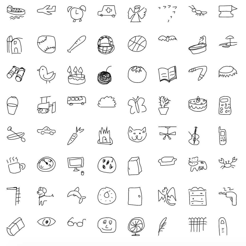
dataset_preview(dataset, image_shape)

Normalize dataset
def normalize_example(example):
    image = example['image']
    label = example['label']

    image = tf.math.divide(image, 255)

    return (image, label)
def augment_example(image, label):
    image = tf.image.random_flip_left_right(image)
    return (image, label)
dataset_normalized = dataset.map(normalize_example).map(augment_example)
for (image, label) in dataset_normalized.take(1):
    class_index = label.numpy()
    class_name = label_index_to_string(class_index)

    print('{} ({})'.format(class_name, class_index), '\n')
    print('Image shape: ', image.shape, '\n')
    print(np.reshape(image.numpy(), (28, 28)), '\n')
backpack (12)

Image shape:  (28, 28, 1)

[[0.         0.         0.         0.         0.         0.
  0.         0.         0.         0.         0.         0.
  0.         0.         0.         0.         0.         0.
  0.         0.         0.         0.         0.         0.
  0.         0.         0.         0.        ]
 [0.         0.         0.         0.         0.         0.
  0.         0.         0.         0.         0.         0.
  0.         0.01176471 0.12156863 0.24705882 0.37254903 0.4509804
  0.3372549  0.19607843 0.00784314 0.         0.         0.
  0.         0.         0.         0.        ]
 [0.         0.         0.         0.         0.         0.29411766
  0.7176471  0.6901961  0.59607846 0.03921569 0.21176471 0.7137255
  0.87058824 0.98039216 1.         1.         1.         1.
  1.         1.         0.90588236 0.5921569  0.23921569 0.
  0.         0.         0.         0.        ]
 [0.         0.         0.         0.         0.5058824  1.
  0.84705883 0.7921569  1.         0.38431373 0.8627451  0.87058824
  0.6156863  0.49019608 0.3647059  0.23529412 0.10980392 0.03137255
  0.14901961 0.32156864 0.63529414 0.9372549  0.99607843 0.42352942
  0.         0.         0.         0.        ]
 [0.         0.         0.         0.12941177 0.98039216 0.61960787
  0.01568628 0.         0.8        0.81960785 1.         0.9254902
  0.4117647  0.         0.         0.         0.         0.
  0.         0.         0.         0.02352941 0.6431373  0.99607843
  0.34509805 0.         0.         0.        ]
 [0.         0.         0.         0.61960787 0.9529412  0.11764706
  0.60784316 0.92156863 0.827451   1.         0.99607843 0.7254902
  1.         0.38039216 0.         0.         0.         0.
  0.         0.         0.         0.         0.01176471 0.75686276
  0.8980392  0.03921569 0.         0.        ]
 [0.         0.         0.14901961 0.9843137  0.5254902  0.6
  0.9843137  0.63529414 0.9882353  0.9607843  0.88235295 0.00392157
  0.7058824  0.94509804 0.02352941 0.         0.         0.
  0.         0.         0.         0.         0.         0.27058825
  1.         0.24313726 0.         0.        ]
 [0.         0.         0.5882353  0.9411765  0.10196079 0.9607843
  0.5686275  0.         0.45490196 1.         0.58431375 0.
  0.29411766 1.         0.22745098 0.         0.         0.
  0.         0.         0.         0.         0.         0.11372549
  1.         0.36862746 0.         0.        ]
 [0.         0.         0.81960785 0.6784314  0.3019608  1.
  0.24313726 0.         0.24313726 1.         0.26666668 0.
  0.05490196 0.9843137  0.47843137 0.         0.         0.
  0.         0.         0.         0.         0.         0.00784314
  0.9764706  0.5019608  0.         0.        ]
 [0.         0.         0.9411765  0.5411765  0.5921569  0.9254902
  0.01568628 0.         0.29803923 1.         0.18039216 0.
  0.         0.8666667  0.6156863  0.         0.         0.
  0.         0.         0.         0.         0.         0.
  0.85490197 0.627451   0.         0.        ]
 [0.         0.         0.9843137  0.49803922 0.7372549  0.7372549
  0.         0.         0.29803923 1.         0.18039216 0.
  0.         0.8352941  0.6431373  0.         0.01568628 0.1764706
  0.         0.         0.         0.         0.         0.
  0.7294118  0.75686276 0.         0.        ]
 [0.         0.01960784 1.         0.45882353 0.78039217 0.6901961
  0.         0.         0.29803923 1.         0.18039216 0.
  0.         0.8039216  0.6784314  0.         0.29411766 0.9843137
  0.03529412 0.         0.17254902 0.6039216  0.00784314 0.
  0.61960787 0.8862745  0.         0.        ]
 [0.         0.05490196 1.         0.42352942 0.81960785 0.6509804
  0.         0.         0.29803923 1.         0.18039216 0.
  0.         0.627451   0.9529412  0.4        0.17254902 0.23921569
  0.13333334 0.13725491 0.38431373 0.78039217 0.5176471  0.6666667
  0.9843137  0.9882353  0.02352941 0.        ]
 [0.         0.09019608 1.         0.3882353  0.8627451  0.6117647
  0.         0.         0.29803923 1.         0.18039216 0.
  0.         0.47058824 0.9764706  1.         1.         1.
  1.         1.         1.         1.         0.96862745 0.8392157
  0.7921569  1.         0.09411765 0.        ]
 [0.         0.06666667 1.         0.42352942 0.8666667  0.63529414
  0.         0.         0.28235295 1.         0.2        0.
  0.         0.5058824  0.96862745 0.12156863 0.32156864 0.33333334
  0.33333334 0.33333334 0.24313726 0.10980392 0.00392157 0.
  0.42352942 1.         0.05098039 0.        ]
 [0.         0.         0.92941177 0.56078434 0.62352943 0.9098039
  0.01176471 0.         0.14901961 1.         0.34117648 0.
  0.         0.5058824  0.96862745 0.         0.         0.
  0.         0.         0.         0.         0.         0.
  0.4745098  0.99215686 0.00784314 0.        ]
 [0.         0.         0.7764706  0.78039217 0.28627452 1.
  0.30588236 0.         0.01568628 0.972549   0.49803922 0.
  0.         0.5058824  0.96862745 0.         0.         0.
  0.07843138 0.24705882 0.15294118 0.03137255 0.         0.
  0.5254902  0.9490196  0.         0.        ]
 [0.         0.         0.3764706  1.         0.39607844 0.8627451
  0.9137255  0.3764706  0.00392157 0.8352941  0.6509804  0.
  0.         0.5058824  0.96862745 0.         0.37254903 0.8
  0.99215686 1.         1.         1.         0.9019608  0.78039217
  0.85490197 0.9098039  0.         0.        ]
 [0.         0.         0.00392157 0.7058824  0.9882353  0.53333336
  0.7411765  1.         0.41568628 0.6784314  0.8117647  0.
  0.         0.5058824  0.96862745 0.         0.9372549  0.89411765
  0.45490196 0.24705882 0.32941177 0.4509804  0.5764706  0.7254902
  1.         0.90588236 0.         0.        ]
 [0.         0.         0.         0.03137255 0.6313726  1.
  0.6392157  0.29803923 0.08627451 0.52156866 0.9647059  0.00784314
  0.         0.5058824  0.96862745 0.         0.7764706  0.69411767
  0.         0.         0.         0.         0.         0.19215687
  1.         0.8627451  0.         0.        ]
 [0.         0.         0.         0.         0.         0.44313726
  0.9843137  0.9490196  0.76862746 0.9411765  1.         0.14509805
  0.         0.5058824  0.96862745 0.         0.8156863  0.65882355
  0.         0.         0.         0.         0.         0.50980395
  0.99607843 0.74509805 0.         0.        ]
 [0.         0.         0.         0.         0.         0.
  0.21960784 0.5529412  0.72156864 0.64705884 0.972549   0.62352943
  0.         0.49411765 0.98039216 0.         0.68235296 0.8784314
  0.05098039 0.         0.         0.         0.         0.85882354
  1.         0.4509804  0.         0.        ]
 [0.         0.         0.         0.         0.         0.
  0.         0.         0.         0.         0.49803922 0.99607843
  0.23529412 0.45490196 1.         0.01960784 0.27058825 0.9882353
  0.9019608  0.3764706  0.00784314 0.         0.18039216 1.
  0.99215686 0.11764706 0.         0.        ]
 [0.         0.         0.         0.         0.         0.
  0.         0.         0.         0.         0.03529412 0.84313726
  0.94509804 0.6313726  1.         0.05882353 0.         0.18039216
  0.74509805 1.         0.80784315 0.6627451  0.95686275 1.
  0.45882353 0.         0.         0.        ]
 [0.         0.         0.         0.         0.         0.
  0.         0.         0.         0.         0.         0.09019608
  0.79607844 1.         1.         0.8980392  0.8509804  0.8
  0.7490196  0.8901961  1.         1.         0.9843137  0.6117647
  0.         0.         0.         0.        ]
 [0.         0.         0.         0.         0.         0.
  0.         0.         0.         0.         0.         0.
  0.00392157 0.42352942 1.         0.7176471  0.62352943 0.6666667
  0.7254902  0.6666667  0.4392157  0.25490198 0.01568628 0.
  0.         0.         0.         0.        ]
 [0.         0.         0.         0.         0.         0.
  0.         0.         0.         0.         0.         0.
  0.         0.01176471 0.38039216 0.09019608 0.         0.
  0.         0.         0.         0.         0.         0.
  0.         0.         0.         0.        ]
 [0.         0.         0.         0.         0.         0.
  0.         0.         0.         0.         0.         0.
  0.         0.         0.         0.         0.         0.
  0.         0.         0.         0.         0.         0.
  0.         0.         0.         0.        ]]
dataset_normalized_preview(dataset_normalized, image_shape)

Prepare Train/Validation/Test dataset splits
# A quick example of how we're going to split the dataset for train/test/validation subsets.
tmp_ds = tf.data.Dataset.range(10)
print('tmp_ds:', list(tmp_ds.as_numpy_iterator()))

tmp_ds_test = tmp_ds.take(2)
print('tmp_ds_test:', list(tmp_ds_test.as_numpy_iterator()))

tmp_ds_val = tmp_ds.skip(2).take(3)
print('tmp_ds_val:', list(tmp_ds_val.as_numpy_iterator()))

tmp_ds_train = tmp_ds.skip(2 + 3)
print('tmp_ds_train:', list(tmp_ds_train.as_numpy_iterator()))
tmp_ds: [0, 1, 2, 3, 4, 5, 6, 7, 8, 9]
tmp_ds_test: [0, 1]
tmp_ds_val: [2, 3, 4]
tmp_ds_train: [5, 6, 7, 8, 9]
# Dataset split
test_dataset_batches = 1
val_dataset_batches = 1

# Dataset batching and shuffling
shuffle_buffer_size = 20000
batch_size = 20000
prefetch_buffer_batches = 10

# Training
epochs = 40
steps_per_epoch = 200
dataset_batched = dataset_normalized \
    .shuffle(
        buffer_size=shuffle_buffer_size,
        reshuffle_each_iteration=True
    ) \
    .batch(batch_size=batch_size)
# TEST dataset.
dataset_test = dataset_batched \
    .take(test_dataset_batches)

# VALIDATION dataset.
dataset_val = dataset_batched \
    .skip(test_dataset_batches) \
    .take(val_dataset_batches)

# TRAIN dataset.
dataset_train = dataset_batched \
    .skip(test_dataset_batches + val_dataset_batches) \
    .prefetch(buffer_size=prefetch_buffer_batches) \
    .repeat()
for (image_test, label_test) in dataset_test.take(1):
    print('label_test.shape: ', label_test.shape)
    print('image_test.shape: ', image_test.shape)

print()

for (image_val, label_val) in dataset_val.take(1):
    print('label_val.shape: ', label_val.shape)
    print('image_val.shape: ', image_val.shape)

print()

for (image_train, label_train) in dataset_train.take(1):
    print('label_train.shape: ', label_train.shape)
    print('image_train.shape: ', image_train.shape)
label_test.shape:  (20000,)
image_test.shape:  (20000, 28, 28, 1)

label_val.shape:  (20000,)
image_val.shape:  (20000, 28, 28, 1)

label_train.shape:  (20000,)
image_train.shape:  (20000, 28, 28, 1)
Create model
model = tf.keras.models.Sequential()

model.add(tf.keras.layers.Flatten(
    input_shape=image_shape
))

model.add(tf.keras.layers.Dense(
    units=512,
    activation=tf.keras.activations.relu
))

model.add(tf.keras.layers.Dense(
    units=512,
    activation=tf.keras.activations.relu
))

model.add(tf.keras.layers.Dense(
    units=512,
    activation=tf.keras.activations.relu
))

model.add(tf.keras.layers.Dense(
    units=num_classes,
    activation=tf.keras.activations.softmax
))
model.summary()
Model: "sequential_44"
_________________________________________________________________
Layer (type)                 Output Shape              Param #
=================================================================
flatten_44 (Flatten)         (None, 784)               0
_________________________________________________________________
dense_148 (Dense)            (None, 512)               401920
_________________________________________________________________
dense_149 (Dense)            (None, 512)               262656
_________________________________________________________________
dense_150 (Dense)            (None, 512)               262656
_________________________________________________________________
dense_151 (Dense)            (None, 345)               176985
=================================================================
Total params: 1,104,217
Trainable params: 1,104,217
Non-trainable params: 0
_________________________________________________________________
tf.keras.utils.plot_model(
    model,
    show_shapes=True,
    show_layer_names=True,
)

adam_optimizer = tf.keras.optimizers.Adam(learning_rate=0.001)

model.compile(
    optimizer=adam_optimizer,
    loss=tf.keras.losses.sparse_categorical_crossentropy,
    metrics=['accuracy']
)
Train model
early_stopping_callback = tf.keras.callbacks.EarlyStopping(
    patience=5,
    monitor='val_accuracy',
    restore_best_weights=True,
    verbose=1
)
training_history = model.fit(
    x=dataset_train,
    epochs=epochs,
    steps_per_epoch=steps_per_epoch,
    validation_data=dataset_val,
    callbacks=[
        early_stopping_callback
    ]
)
Train for 200 steps
Epoch 1/40
200/200 [==============================] - 800s 4s/step - loss: 3.6174 - accuracy: 0.2604 - val_loss: 2.9169 - val_accuracy: 0.3690
Epoch 2/40
200/200 [==============================] - 739s 4s/step - loss: 2.7120 - accuracy: 0.4023 - val_loss: 2.5463 - val_accuracy: 0.4383
Epoch 3/40
200/200 [==============================] - 992s 5s/step - loss: 2.4390 - accuracy: 0.4517 - val_loss: 2.3391 - val_accuracy: 0.4702
Epoch 4/40
200/200 [==============================] - 1005s 5s/step - loss: 2.2781 - accuracy: 0.4817 - val_loss: 2.2136 - val_accuracy: 0.4935
Epoch 5/40
200/200 [==============================] - 1019s 5s/step - loss: 2.1720 - accuracy: 0.5025 - val_loss: 2.1351 - val_accuracy: 0.5098
Epoch 6/40
200/200 [==============================] - 809s 4s/step - loss: 2.0922 - accuracy: 0.5180 - val_loss: 2.0502 - val_accuracy: 0.5277
Epoch 7/40
200/200 [==============================] - 812s 4s/step - loss: 2.0288 - accuracy: 0.5304 - val_loss: 1.9968 - val_accuracy: 0.5404
Epoch 8/40
200/200 [==============================] - 801s 4s/step - loss: 1.9788 - accuracy: 0.5407 - val_loss: 1.9287 - val_accuracy: 0.5498
Epoch 9/40
200/200 [==============================] - 935s 5s/step - loss: 1.9373 - accuracy: 0.5488 - val_loss: 1.8987 - val_accuracy: 0.5552
Epoch 10/40
200/200 [==============================] - 971s 5s/step - loss: 1.9007 - accuracy: 0.5565 - val_loss: 1.8762 - val_accuracy: 0.5566
Epoch 11/40
200/200 [==============================] - 804s 4s/step - loss: 1.8710 - accuracy: 0.5624 - val_loss: 1.8370 - val_accuracy: 0.5676
Epoch 12/40
200/200 [==============================] - 849s 4s/step - loss: 1.8443 - accuracy: 0.5681 - val_loss: 1.8345 - val_accuracy: 0.5700
Epoch 13/40
200/200 [==============================] - 786s 4s/step - loss: 1.8210 - accuracy: 0.5722 - val_loss: 1.8026 - val_accuracy: 0.5753
Epoch 14/40
200/200 [==============================] - 811s 4s/step - loss: 1.7958 - accuracy: 0.5777 - val_loss: 1.7607 - val_accuracy: 0.5817
Epoch 15/40
200/200 [==============================] - 834s 4s/step - loss: 1.7778 - accuracy: 0.5816 - val_loss: 1.7695 - val_accuracy: 0.5829
Epoch 16/40
200/200 [==============================] - 952s 5s/step - loss: 1.7592 - accuracy: 0.5852 - val_loss: 1.7420 - val_accuracy: 0.5882
Epoch 17/40
200/200 [==============================] - 814s 4s/step - loss: 1.7429 - accuracy: 0.5885 - val_loss: 1.7143 - val_accuracy: 0.5917
Epoch 18/40
200/200 [==============================] - 955s 5s/step - loss: 1.7256 - accuracy: 0.5921 - val_loss: 1.7113 - val_accuracy: 0.5965
Epoch 19/40
200/200 [==============================] - 807s 4s/step - loss: 1.7141 - accuracy: 0.5948 - val_loss: 1.6815 - val_accuracy: 0.6019
Epoch 20/40
200/200 [==============================] - 816s 4s/step - loss: 1.7011 - accuracy: 0.5973 - val_loss: 1.6910 - val_accuracy: 0.6006
Epoch 21/40
200/200 [==============================] - 841s 4s/step - loss: 1.6860 - accuracy: 0.6003 - val_loss: 1.6776 - val_accuracy: 0.5995
Epoch 22/40
200/200 [==============================] - 1008s 5s/step - loss: 1.6748 - accuracy: 0.6027 - val_loss: 1.6483 - val_accuracy: 0.6089
Epoch 23/40
200/200 [==============================] - 935s 5s/step - loss: 1.6659 - accuracy: 0.6043 - val_loss: 1.6715 - val_accuracy: 0.6015
Epoch 24/40
200/200 [==============================] - 809s 4s/step - loss: 1.6566 - accuracy: 0.6064 - val_loss: 1.6618 - val_accuracy: 0.6066
Epoch 25/40
200/200 [==============================] - 940s 5s/step - loss: 1.6460 - accuracy: 0.6084 - val_loss: 1.6429 - val_accuracy: 0.6059
Epoch 26/40
200/200 [==============================] - 1005s 5s/step - loss: 1.6382 - accuracy: 0.6100 - val_loss: 1.5783 - val_accuracy: 0.6209
Epoch 27/40
200/200 [==============================] - 1000s 5s/step - loss: 1.6275 - accuracy: 0.6123 - val_loss: 1.6208 - val_accuracy: 0.6143
Epoch 28/40
200/200 [==============================] - 975s 5s/step - loss: 1.6214 - accuracy: 0.6138 - val_loss: 1.6122 - val_accuracy: 0.6130
Epoch 29/40
200/200 [==============================] - 824s 4s/step - loss: 1.6127 - accuracy: 0.6153 - val_loss: 1.6137 - val_accuracy: 0.6143
Epoch 30/40
200/200 [==============================] - 903s 5s/step - loss: 1.6070 - accuracy: 0.6168 - val_loss: 1.5767 - val_accuracy: 0.6190
Epoch 31/40
199/200 [============================>.] - ETA: 4s - loss: 1.6007 - accuracy: 0.6184Restoring model weights from the end of the best epoch.
200/200 [==============================] - 820s 4s/step - loss: 1.6006 - accuracy: 0.6184 - val_loss: 1.6009 - val_accuracy: 0.6187
Epoch 00031: early stopping
# Renders the charts for training accuracy and loss.
def render_training_history(training_history):
    loss = training_history.history['loss']
    val_loss = training_history.history['val_loss']

    accuracy = training_history.history['accuracy']
    val_accuracy = training_history.history['val_accuracy']

    plt.figure(figsize=(14, 4))

    plt.subplot(1, 2, 1)
    plt.title('Loss')
    plt.xlabel('Epoch')
    plt.ylabel('Loss')
    plt.plot(loss, label='Training set')
    plt.plot(val_loss, label='Test set', linestyle='--')
    plt.legend()
    plt.grid(linestyle='--', linewidth=1, alpha=0.5)

    plt.subplot(1, 2, 2)
    plt.title('Accuracy')
    plt.xlabel('Epoch')
    plt.ylabel('Accuracy')
    plt.plot(accuracy, label='Training set')
    plt.plot(val_accuracy, label='Test set', linestyle='--')
    plt.legend()
    plt.grid(linestyle='--', linewidth=1, alpha=0.5)

    plt.show()
render_training_history(training_history)

Evaluate model accuracy
Training set accuracy
%%capture
train_loss, train_accuracy = model.evaluate(dataset_train.take(1))
print('Train loss: ', '{:.2f}'.format(train_loss))
print('Train accuracy: ', '{:.2f}'.format(train_accuracy))
Train loss:  1.62
Train accuracy:  0.61
Validation set accuracy
%%capture
val_loss, val_accuracy = model.evaluate(dataset_val)
print('Validation loss: ', '{:.2f}'.format(val_loss))
print('Validation accuracy: ', '{:.2f}'.format(val_accuracy))
Validation loss:  1.63
Validation accuracy:  0.61
Test set accuracy
%%capture
test_loss, test_accuracy = model.evaluate(dataset_test)
print('Test loss: ', '{:.2f}'.format(test_loss))
print('Test accuracy: ', '{:.2f}'.format(test_accuracy))
Test loss:  1.63
Test accuracy:  0.61
Save the model
We will save the entire model to a HDF5 file. The .h5 extension of the file indicates that the model should be saved in Keras format as HDF5 file. To use this model on the front-end we will convert it (later in this notebook) to Javascript understandable format (tfjs_layers_model with .json and .bin files) using tensorflowjs_converter as it is specified in the main README.
model_name = 'sketch_recognition_mlp.h5'
model.save(model_name, save_format='h5')
Converting the model to web-format
To use this model on the web we need to convert it into the format that will be understandable by tensorflowjs. To do so we may use tfjs-converter as following:
tensorflowjs_converter --input_format keras \
  ./experiments/sketch_recognition_mlp/sketch_recognition_mlp.h5 \
  ./demos/public/models/sketch_recognition_mlp
You find this experiment in the Demo app and play around with it right in you browser to see how the model performs in real life.