#reveal configuration
from notebook.services.config import ConfigManager
cm = ConfigManager()
cm.update('livereveal', {
        'theme': 'white',
        'transition': 'none',
        'controls': 'false',
        'progress': 'true',
})

import tensorflow as tf
import numpy as np

%load_ext tikzmagic
%%javascript
require(['base/js/utils'],
function(utils) {
   utils.load_extensions('calico-spell-check', 'calico-document-tools', 'calico-cell-tools');
});
%%html
<style>
.red { color: #E41A1C; }
.orange { color: #FF7F00 }
.yellow { color: #FFC020 }
.green { color: #4DAF4A }
.blue { color: #377EB8; }
.purple { color: #984EA3 }

#for reveal
.aside .controls, .reveal .controls {
    display: none !important;
    width: 0px !important;
    height: 0px !important;
}

.rise-enabled .reveal .slide-number {
    right: 25px;
    bottom: 25px;
    font-size: 200%;
    color: #377EB8;
}

.rise-enabled .reveal .progress span {
    background: #377EB8;
}

.present .top {
    position: fixed !important;
    top: 0 !important;
}
</style>
Deep Learning for Natural Language Processing
In this chapter we will look into applications of Recurrent Neural Networks (RNNs) for NLP. Deep Learning and RNNs are currently used in many tasks, for instance, machine translation, machine comprehension, question answering, text summarization and generation. In this chapter we take recognizing textual entailment (RTE) as an example task and further look into several tools that help training RNNs for this task.
Outline
- Use-case: Recognizing Textual Entailment
- Conditional Encoding
- Attention
- Bag of Tricks
- Continuous Optimization
- Regularization
- Hyper-parameter Optimization
- Pre-trained Representations
- Batching
- Bucketing
- TensorFlow
dynamic_rnn - Bi-directional RNNs
Recognizing Textual Entailment (RTE)
RTE is the task of determining the logical relationship between two natural language sentences. Although this can be simply seen as a classification problem, it is a very difficult task as it needs commonsense and background knowledge about the world, some understanding of natural language, as well a form of fine-grained reasoning.
- A wedding party is taking pictures
- There is a funeral : Contradiction
- They are outside : Neutral
- Someone got married : Entailment
State of the Art until 2015
[Lai and Hockenmaier, 2014, Jimenez et al., 2014, Zhao et al., 2014, Beltagy et al., 2015 etc.]
- Engineered natural language processing pipelines
- Various external resources
- Specialized subcomponents
- Extensive manual creation of features:
- Negation detection, word overlap, part-of-speech tags, dependency parses, alignment, unaligned matching, chunk alignment, synonym, hypernym, antonym, denotation graph
Neural Networks for RTE
As shown above, models for RTE heavily relied on engineered features. One reason why neural networks were not applied to this task is due to the absence of high-quality large-scale RTE corpora.
Previous RTE corpora:
- Tiny data sets (1k-10k examples)
- Partly synthetic examples
Stanford Natural Inference Corpus (SNLI):
- 500k sentence pairs
- Two orders of magnitude larger than existing RTE data set
- All examples generated by humans
Independent Sentence Encoding
With the introduction of a large-scale RTE corpora, neural networks became feasible to train. A first baseline model by Bowman et al. (2015) used LSTMs to encode the premise and hypothesis independently of each other.
[Bowman et al, 2015]
Same LSTM encodes premise and hypothesis

Independent Sentence Encoding
The way RNNs can encode a sentence is to apply the RNN to the sequence of tokens and subsequently take the last output vector as the representation of the sentence. After training the RNN, the hope is that this last output vector would capture the semantics of the sentence that is needed for solving the downstream task (RTE in this case).
[Bowman et al, 2015]
Same LSTM encodes premise and hypothesis

You can’t cram the meaning of a whole
%&!$# sentence into a single $&!#* vector!
-- Raymond J. Mooney
The problem with this approach is that encoding a whole sentence into a single dense vector has obvious representational limitations. However, it is a simple model that sometimes works surprisingly well in practice and often serves as a baseline for more complex architectures.
Independent Sentence Encoding
Once both sentences are encoded as vectors, we can use a multi-layer perceptron followed by a softmax to model the probability of each class (entailment, neutral, contradiction) given the two sentences.
[Bowman et al, 2015]

TensorFlow: Multi-layer Perceptron
Below we show simple TensorFlow code for a multi-layer perceptron. Note that we sample two random sentence representations, whereas in practice we would use the output of an RNN as explained earlier.
with tf.Graph().as_default():
    def mlp(input_vector, layers=3, hidden_dim=200, output_dim=3):
        # [input_size] => [input_size x 1] (column vector)
        tmp = tf.expand_dims(input_vector, 1)
        for i in range(layers+1):
            W = tf.get_variable(
                "W_"+str(i), [hidden_dim, hidden_dim])
            # tanh(Wx^T)
            tmp = tf.tanh(tf.matmul(W, tmp))
        W = tf.get_variable(
            "W_"+str(layers+1), [output_dim, hidden_dim])
        # [input_size x 1] => [input_size]
        return tf.squeeze(tf.matmul(W, tmp))
    premise = tf.placeholder(tf.float32, [None], "premise")
    hypothesis = tf.placeholder(tf.float32, [None], "hypothesis")
    output = tf.nn.softmax(mlp(tf.concat([premise, hypothesis], axis=0)))
    # in practice: outputs of an LSTM
    v1 = np.random.rand(100); v2 = np.random.rand(100)
    with tf.Session() as sess:
        sess.run(tf.global_variables_initializer())
        print(sess.run(output, {premise: v1, hypothesis: v2}))
[ 0.28892419 0.30673885 0.40433696]
Results
| Model | k | θW+M | θM | Train | Dev | Test |
|---|---|---|---|---|---|---|
| LSTM [Bowman et al.] | 100 | $\approx$10M | 221k | 84.4 | - | 77.6 |
| Classifier [Bowman et al.] | - | - | - | 99.7 | - | 78.2 |
In fact, this simple way of encoding the relationship between two sentences is still inferior compared to a classifier with hand-engineered features. Next, we will investigate slightly more complex models.
Conditional Endcoding

If we think more about the problem, it does not seem natural to encode both sentences independently. Instead, the way we read the hypothesis could be influenced by our understanding of the premise. For designing a model we could thus use two LSTMs, one for the premise and one for the hypothesis, where the initial state of the hypothesis model is initialized by the hidden state of the premise model.
Instead of a concatenation of the premise and hypothesis representation, we now simply project the last output representation into the space of the three target classes and apply the softmax function.
Conditional Endcoding

This has the advantage that we do not need to encode both sentences as fixed vector representations anymore. While the premise still needs to be encoded (last hidden state, $\mathbf{c}_5$), the LSTM used for the hypothesis can use all its parameters to track the state of the sequence comparison for the final prediction.
Results
| Model | k | θW+M | θM | Train | Dev | Test |
|---|---|---|---|---|---|---|
| LSTM [Bowman et al.] | 100 | $\approx$10M | 221k | 84.4 | - | 77.6 |
| Classifier [Bowman et al.] | - | - | - | 99.7 | - | 78.2 |
| Conditional Endcoding | 159 | 3.9M | 252k | 84.4 | 83.0 | 81.4 |
Attention [Graves 2013, Bahdanau et al. 2015]

Conditional encoding improves generalization compared to independent encoding of premise and hypothesis. Another improvement can be achieved by using a neural attention mechanism. To this end we compare the last output vector ($\mathbf{h}_N$) with all premise output vectors (concatenated to $\mathbf{Y}$) and model a probability distribution $\alpha$ over premise output vectors using a softmax. Lastly, we obtain a context representation $\mathbf{r}$ by weighting output vectors with the attention $\alpha$, and use that context representation together with $\mathbf{h}_N$ for prediction.
Attention [Graves 2013, Bahdanau et al. 2015]

The main benefit of attention is that we avoid encoding the entire premise in a single vector.

Contextual Understanding

Results
| Model | k | θW+M | θM | Train | Dev | Test |
|---|---|---|---|---|---|---|
| LSTM [Bowman et al.] | 100 | $\approx$10M | 221k | 84.4 | - | 77.6 |
| Classifier [Bowman et al.] | - | - | - | 99.7 | - | 78.2 |
| Conditional Encoding | 159 | 3.9M | 252k | 84.4 | 83.0 | 81.4 |
| Attention | 100 | 3.9M | 242k | 85.4 | 83.2 | 82.3 |
Fuzzy Attention

Word-by-word Attention [Bahdanau et al. 2015, Hermann et al. 2015, Rush et al. 2015]

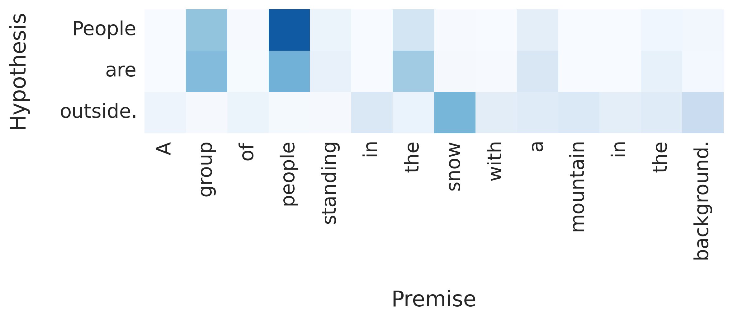
An extension to the attention mechanism described above is to allow the model to attend over premise output vectors for every word in the hypothesis. This can be achieved by a small adaption of the previous model.
Word-by-word Attention [Bahdanau et al. 2015, Hermann et al. 2015, Rush et al. 2015]

Reordering
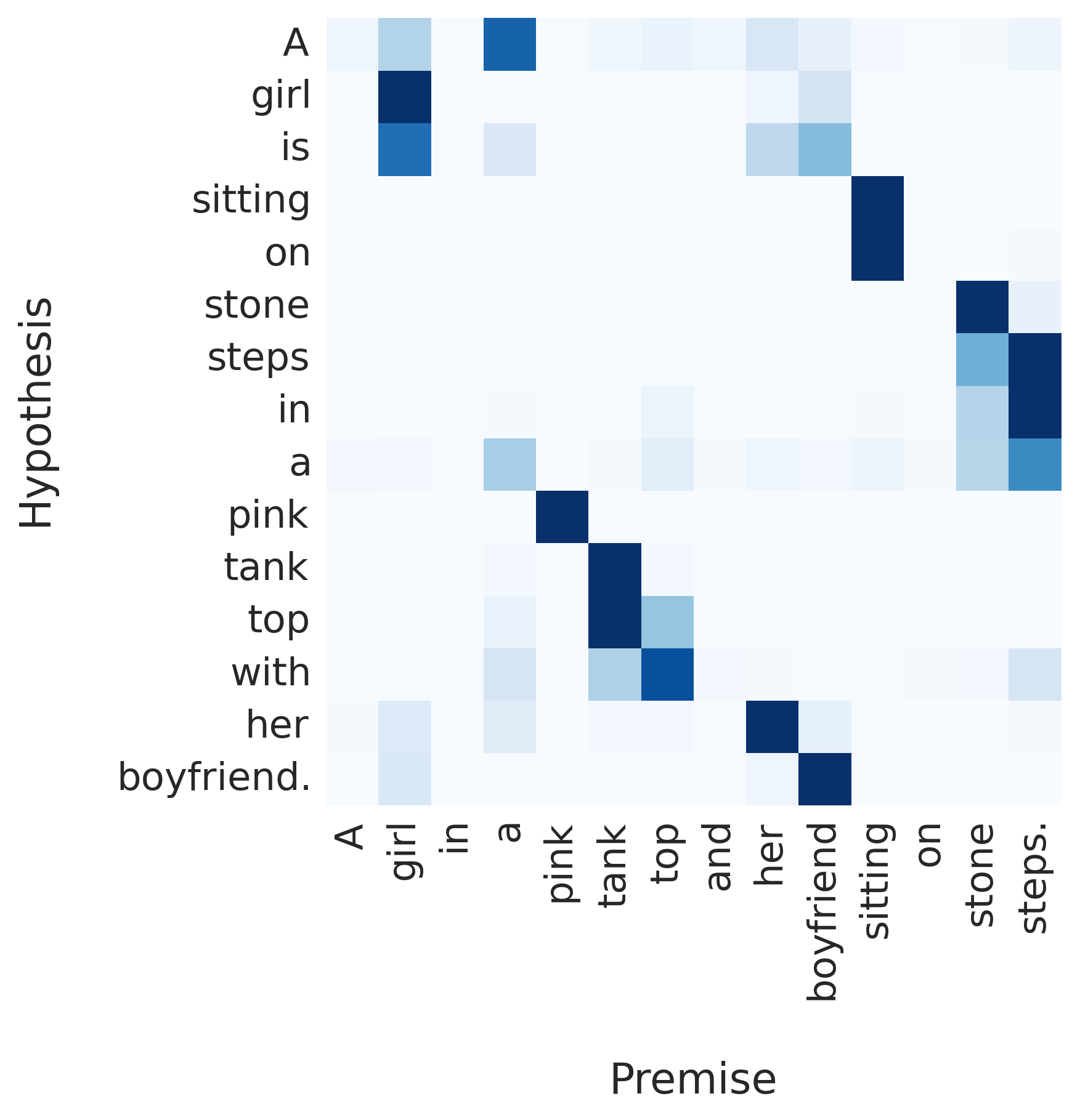
Garbage Can = Trashcan

Kids = Girl + Boy

Snow is outside
Results
| Model | k | θW+M | θM | Train | Dev | Test |
|---|---|---|---|---|---|---|
| LSTM [Bowman et al.] | 100 | $\approx$10M | 221k | 84.4 | - | 77.6 |
| Classifier [Bowman et al.] | - | - | - | 99.7 | - | 78.2 |
| Conditional Encoding | 159 | 3.9M | 252k | 84.4 | 83.0 | 81.4 |
| Attention | 100 | 3.9M | 242k | 85.4 | 83.2 | 82.3 |
| Word-by-word Attention | 100 | 3.9M | 252k | 85.3 | 83.7 | 83.5 |
Bag of Tricks
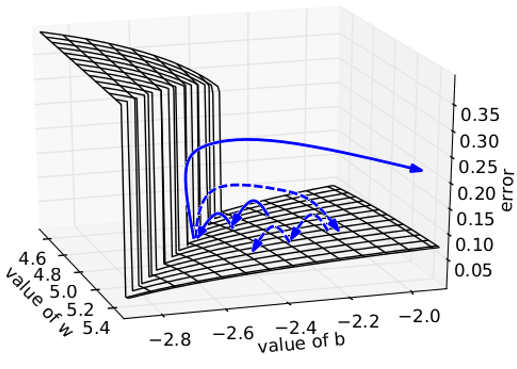
Continuous Optimization
 Source: Wikipedia
Momentum

TensorFlow: Optimizers
- GradientDescent
- RMSProp
- Adagrad
- Adadelta
- Adam
with tf.Graph().as_default():
    x = tf.get_variable("param", [])
    loss = -tf.log(tf.sigmoid(x))  # dummy example
    optim = tf.train.AdamOptimizer(learning_rate=0.1)
    min_op = optim.minimize(loss)
    with tf.Session() as sess:
        sess.run(tf.global_variables_initializer())
        sess.run(x.assign(1.5))
        for i in range(10):
            print(sess.run([min_op, loss], {})[1])
0.201413
0.183901
0.167832
0.153134
0.139727
0.127529
0.116455
0.106421
0.0973447
0.0891449
There are various gradient based optimizers that you can use in TensorFlow. We recommend Adam with an initial learning rate of $0.1$ or $0.01$.
Gradient Clipping
with tf.Graph().as_default():
    x = tf.get_variable("param", [])
    loss = -tf.log(tf.sigmoid(x))  # dummy example
    optim = tf.train.AdamOptimizer(learning_rate=0.1)
    gradients = optim.compute_gradients(loss)
    capped_gradients = \
        [(tf.clip_by_value(grad, -0.1, 0.1), var) for grad, var in gradients]
    min_op = optim.apply_gradients(capped_gradients)
    with tf.Session() as sess:
        sess.run(tf.global_variables_initializer()); sess.run(x.assign(1.5))
        for i in range(100):
            if i % 10 == 0:
                grads = sess.run([min_op, gradients, capped_gradients], {})[1:]
                print(" => ".join([str(grad[0][0]) for grad in grads]))
-0.182426 => -0.1
-0.167982 => -0.1
-0.154465 => -0.1
-0.141851 => -0.1
-0.130109 => -0.1
-0.119203 => -0.1
-0.109097 => -0.1
-0.0997508 => -0.0997508
-0.0911243 => -0.0911243
-0.0832129 => -0.0832129
For more stable training, gradient clipping is often applied. It simply caps gradients at a predefined interval, or in the case of tf.clip_by_norm, constrains the norm of the gradient.
Regularization

with tf.Graph().as_default():
    x = tf.placeholder(tf.float32, [None], "input")
    x_dropped = tf.nn.dropout(x, 0.7)  # keeps 70% of values

    with tf.Session() as sess:
        print(sess.run(x_dropped, {x: np.random.rand(6)}))
[ 0. 0.40834624 1.31100929 0. 1.08233535 0. ]
One of the most successful regularization techniques is dropout. The idea is to randomly set output representations to $0$ at every execution of the computation graph. By repeating this produce, we are effectively averaging over different model architectures (see Fig b) and increase the robustness of the model. Common dropout values are $0.1$ or $0.2$, i.e., keeping 90% or 80% of the values in the output representation respectively.
Early Stopping

Another simple way of regularization is to stop training on the training set (blue) once overfitting on a dev set (red) occurs.
Hyper-parameter Optimization
[Bergstra and Bengio 2012]
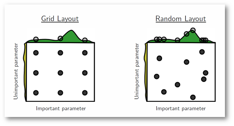
We often use grid search for finding a good combination of model hyper-parameters on a dev set. However, it turns out that a more effective method is random search by sampling uniform values for the hyper-parameters from a predefined interval.
Pre-trained Representations
with tf.Graph().as_default():
    vocab_size = 4; embedding_size = 3
    W = tf.get_variable("W", [vocab_size, embedding_size], trainable=False)
    W = W.assign(np.array([[0, 1, 2], [3, 4, 5], [6, 7, 8], [9, 10, 11]]))
    seq =  tf.placeholder(tf.int64, [None], "seq")
    seq_embedded = tf.nn.embedding_lookup(W, seq)
    with tf.Session() as sess:
        sess.run(tf.global_variables_initializer())
        print(sess.run(seq_embedded, {seq:[0, 3, 2, 3, 1]})[2])
[ 6. 7. 8.]
Instead of training task-specific word representations, it is sometimes helpful to use pre-trained word vectors from word2vec or GloVe. Above, you can find a simply example of manually setting vectors of a word embedding matrix. Note that by setting trainable=False, the model cannot update these word embeddings during training. If we only want to use pre-trained word vectors as initializer so that we can fine-tune them based on our task, we would need set trainable=True.
Projecting Representations
with tf.Graph().as_default():
    vocab_size = 4; embedding_size = 3; input_size = 2
    W = tf.get_variable("W", [vocab_size, embedding_size], trainable=False)
    W = W.assign(np.array([[0, 1, 2], [3, 4, 5], [6, 7, 8], [9, 10, 11]]))
    seq =  tf.placeholder(tf.int64, [None], "seq")
    seq_embedded = tf.contrib.layers.linear(tf.nn.embedding_lookup(W, seq), input_size)
    with tf.Session() as sess:
        sess.run(tf.global_variables_initializer())
        print(sess.run(seq_embedded, {seq:[0, 3, 2, 3, 1]})[2])
[-13.46509552 2.99458957]
Sometimes we want to work with pre-trained word vectors (e.g. $300$ dimensional word2vec vectors), but use a different hidden size for our RNN. We can learn a linear projection from one vector space to another via tf.contrib.layers.linear. If we want to use a non-linear projection, we can simply call a non-linear function like tanh on the output of linear.

Batching is used to maximize utilization of GPUs. However, even if you run your models on CPUs, linear algebra libraries often can make use of batched computations. Furthermore, batching is needed for batch gradient descent. The idea is simple: instead of processing a single example such as a sequence of word vectors (represented as $N \times k$ matrix above), we are going to process many of these at the same time (represented by the $mb \times N \times k$ order-3 tensor).

When batching sequences, we will generally have sequences of different lengths in one batch. This is wasting computation on padding symbols of the shorter sequence. Hence, it is a good idea to divide training sequences up into buckets of roughly the same sequence length.

with tf.Graph().as_default():
    input_size = 2; output_size = 3; batch_size = 5; max_length = 7
    cell = tf.nn.rnn_cell.LSTMCell(output_size)
    input_embedded = tf.placeholder(tf.float32, [None, None, input_size], "input_embedded")
    input_length = tf.placeholder(tf.int64, [None], "input_length")
    outputs, states = \
        tf.nn.dynamic_rnn(cell, input_embedded, sequence_length=input_length, dtype=tf.float32)
    with tf.Session() as sess:
        sess.run(tf.global_variables_initializer())
        print(sess.run(states, {
                    input_embedded: np.random.randn(batch_size, max_length, input_size),
                    input_length: np.random.randint(1, max_length, batch_size)
                }).h)
[[-0.02504479  0.01778306  0.06259364]
 [-0.39973924  0.15913689 -0.24309666]
 [ 0.1272437  -0.11015443  0.27061945]
 [-0.16756612  0.08985849 -0.09469282]
 [-0.31299666  0.21844    -0.0656506 ]]
We encourage you to use dynamic_rnn for RNNs in TensorFlow. They avoid changes to the hidden state of the RNN once padding symbols are processed. Note that this is orthogonal to bucketing and dynamic_rnn still benefits from grouping sequences of similar length together in one batch.

Many current RNN systems use bidirectional RNNs to incorporate left-hand as well as right-hand side contexts into output representations. To this end, two independent RNNs are executed, one on the normal input sequence and one on its revers. TensorFlow is making this easy via tf.nn.bidirectional_dynamic_rnn.