Denoising Diffusion Probabilistic Models
- In this tutorial, we will cover:
- Preliminaries
- Markovian processes
- Example: one-dimensional random walk
- Properties of Markovian processes
- DDPMs:
- Forward and reverse diffusion
- Loss function (ELBO strikes again)
- Revisiting the noise reversal process
- Training and sampling
- Noise recovery model
- Putting it all together...
In [1]:
import torch
from torchvision import transforms
from torch.utils.data import DataLoader
import numpy as np
import torchvision
from tqdm import tqdm
import matplotlib.pyplot as plt
device = "cuda" if torch.cuda.is_available() else "cpu"
IMG_SIZE = 64
BATCH_SIZE = 128
def load_transformed_dataset():
data_transforms = [
transforms.Resize((IMG_SIZE, IMG_SIZE)),
transforms.RandomHorizontalFlip(),
transforms.ToTensor(), # Scales data into [0,1]
transforms.Lambda(lambda t: (t * 2) - 1) # Scale between [-1, 1]
]
data_transform = transforms.Compose(data_transforms)
data = torchvision.datasets.FashionMNIST(root=".", download=True, transform=data_transform)
return data
def show_tensor_image(image):
reverse_transforms = transforms.Compose([
transforms.Lambda(lambda t: (t + 1) / 2),
transforms.Lambda(lambda t: t.permute(1, 2, 0)), # CHW to HWC
transforms.Lambda(lambda t: t * 255.),
transforms.Lambda(lambda t: t.numpy().astype(np.uint8)),
transforms.ToPILImage(),
])
plt.imshow(reverse_transforms(image),cmap="gray")
data = load_transformed_dataset()
dataloader = DataLoader(dataset=data, batch_size=BATCH_SIZE, shuffle=True, drop_last=True)
Preliminaries
- A discrete time random process is a sequence of random variables:
- We say that a discrete time random process satisfies the Markovian property if:
- Notable example: one dimensional random walk:

And: $$ X_{k+1} | X_k = \begin{cases} X_k+1 & \text{w.p } p \\ X_k-1 & \text{w.p } 1-p \end{cases} $$
- Properties of Markovian processes:
- Generalized Markovian property:
- For every $i_1 < i_2 < ... < i_n < i_{n+1}$:
- Generalized Markovian property:
* Decomposition of the joint distribution:
* Computing expectations and variances via total expectation and variance laws:
* **Law of total expectation:** $\mathbb{E}[X_{k+1}] = \mathbb{E}_{X_k}[\mathbb{E}[X_{k+1}|X_k]]$
+ In the random walk example: $\mathbb{E}[X_{k+1}] = \mathbb{E}_{X_k}[p\cdot(X_k+1)+(1-p)\cdot(X_k-1)] = \mathbb{E}[X_k] + 2p-1$
+ And hence $\mathbb{E}[X_t] = t\cdot(2p-1)$
* **Law of total Variance:** $Var(X_{k+1}) = \mathbb{E}_{X_k}[Var(X_{k+1}|X_k)] + Var_{X_k}(\mathbb{E}[X_{k+1}|X_k]) $
+ Exercise: compute the variance of each timestep in the random walk example.
Denoising Diffusion Probabilistic Models (DDPMs)
- Diffusion Models are physics inspired models that were first introduced by Sohl-Dickstein et. al back in 2015.
- However, they got broadly popularized by Ho et. al in 2020 which showed that DDPMs can outperform state-of-the-art GANs.
The forward and the reverse process
- Idea: Maintain multiple latent variables $x_1,...,x_T$.
- incrementally add noise to the instance $x_0 \sim q(x_0)$ over $T$ steps in a forward process $q(x_t|x_{t-1})$
- Learn to recover the image in a reverse process $p_\theta(x_{t-1}|x_t)$ where the prior is $p_\theta(x_T) \sim \mathcal{N}(\mathbf{0},\mathbf{I})$

- The forward process:
- Unlike, VAEs this is a non-learnable markovian process in which the noise is gardually added.
- The distribution of the data is: $x_0 \sim q(x_0)$.
- Noise is added as follows: $q(x_t|x_{t-1}) := \mathcal{N}(x_t;\sqrt{1-\beta_t}x_{t-1}, \beta_t \mathbf{I})$.
- $\beta_t > 0$ is a scalar hyperparameter refered to as the variance schedule.
In [2]:
def variance_schedule(start, timesteps, stop=None, scheduling_strategy='constant'):
if scheduling_strategy == 'constant':
betas = torch.ones(timesteps) * start
elif scheduling_strategy == 'linear':
betas = torch.linspace(start, stop, timesteps)
else:
raise NotImplementedError
return betas.to(device)
T = 2000
betas = variance_schedule(start=1e-4, timesteps=T, stop=2e-2, scheduling_strategy='linear')
- A very important property of the forward process is that $q(x_t|x_0)$ can be computed directly:
- where $\alpha_t := 1- \beta_t$ and $\bar{\alpha_t} = \prod_{t=1}^T \alpha_t$.
- Exercise: prove this.
In [3]:
import torch.nn.functional as F
# Pre-calculate different terms for closed form
alphas = (1. - betas).to(device)
cum_alphas = torch.cumprod(alphas, dim=0).to(device)
cum_alphas_prev = F.pad(cum_alphas[:-1], (1, 0), value=1.0).to(device)
sqrt_recip_alphas = torch.sqrt(1.0 / alphas).to(device)
sqrt_cum_alphas = torch.sqrt(cum_alphas).to(device)
sqrt_one_minus_cum_alphas = torch.sqrt(1. - cum_alphas).to(device)
posterior_variance = (betas * (1. - cum_alphas_prev) / (1. - cum_alphas)).to(device)
def extract(v, t, x_shape):
"""
Extract some coefficients at specified timesteps, then reshape to
[batch_size, 1, 1, 1, 1, ...] for broadcasting purposes.
"""
out = torch.gather(v, index=t, dim=0).float()
return out.view([t.shape[0]] + [1] * (len(x_shape) - 1))
- With these we can implement the direct sampling of $x_t$ given $x_0$ and $t$:
In [4]:
def direct_sampling(x_0, t):
eps = torch.randn_like(x_0).to(device)
sqrt_cum_alphas_t = extract(sqrt_cum_alphas, t, x_0.shape)
sqrt_one_minus_cum_alphas_t = extract(sqrt_one_minus_cum_alphas, t, x_0.shape)
x_t = sqrt_cum_alphas_t * x_0 + sqrt_one_minus_cum_alphas_t * eps
return x_t, eps
- Let's simulate the forward diffusion process!
In [5]:
# Simulate forward diffusion
x_0 = next(iter(dataloader))[0]
x_0 = x_0[0].to(device) # Take the first image in the first batch
plt.figure(figsize=(15,15))
num_images = 10
stepsize = int(T/num_images)
for idx in range(0, T, stepsize):
plt.subplot(1, num_images+1, int(idx/stepsize) + 1)
plt.gca().title.set_text(f't = {idx}')
plt.gca().axis('off')
t = torch.Tensor([idx]).type(torch.long).to(device)
img, _ = direct_sampling(x_0, t)
img = img.to(device)
show_tensor_image(img.cpu())

- Notice how the SNR will decrease over time.
In [6]:
time = torch.linspace(start=0, end=T, steps=T)
signal = sqrt_cum_alphas.clone().cpu()
noise = sqrt_one_minus_cum_alphas.clone().cpu()
snr = signal / noise
plt.plot(time, signal, c='g', label='signal')
plt.plot(time, noise, c='r', label='noise')
plt.xlabel('time')
plt.ylabel('magnitude')
plt.legend()
Out[6]:
<matplotlib.legend.Legend at 0x7f5f7a063cd0>

In [7]:
plt.xlabel('time')
plt.ylabel('SNR')
plt.plot(time, snr, c='b', label='snr')
plt.yscale('log')

- The reverse process:
- Similiarly to VAEs, this is a learnable markovian process in which the noise is gardually removed.
- The distribution of the final latent variable is standard normal: $x_T \sim p_\theta(x_T) = \mathcal{N}(x_T; \mathbf{0}, \mathbf{I})$.
- Noise is removed as follows: $p_\theta(x_{t-1}|x_t) := \mathcal{N}(x_{t-1};\mathbf{\mu_\theta}(x_t,t), \mathbf{\Sigma_\theta}(x_t,t))$.
- We will revisit the noise removal mechanism design later in this tutorial...
ELBO loss strikes again
To optimize diffusion models we would maximize the log-likelihood $\log p_\theta(x_0)$ by maximizing the ELBO loss, similiarly to VAEs:
$$ \log p_\theta(x_0) = \mathbb{E}_q[\log(\frac{q(x_{1:T}|x_0)}{p_\theta(x_{1:T}|x_0)} \cdot \frac{p_\theta(x_{0:T})}{q(x_{1:T}|x_0)})] = D_{KL}(q(x_{1:T}|x_0) || p_\theta(x_{1:T}|x_0)) + \mathbb{E}_q[\log \frac{p_\theta(x_{0:T})}{q(x_{1:T}|x_0)}]$$And so the ELBO is: $$ \mathcal{L}(\theta;x_0) = \mathbb{E}_q[\log \frac{p_\theta(x_{0:T})}{q(x_{1:T}|x_0)}] = \mathbb{E}_q[\log p(x_T) + \sum_{t \geq 1} \log \frac{p_\theta(x_{t-1}|x_t)}{q(x_t|x_{t-1})}]$$ Which can be written also as: $$ \mathcal{L}(\theta;x_0) = -D_{KL}(q(x_T|x_0) || p_\theta(x_T)) - \sum_{t>1} \mathbb{E}_q[D_{KL}(q(x_{t-1}|x_t,x_0)||p_\theta(x_{t-1}] + \mathbb{E}_q [\log p_\theta(x_0|x_1)]$$
Interpreting the terms in the ELBO:
- The first term $L_T$ is analogous to the latent space regularization in VAEs, however in our setting it is constant (why?).
- The terms in the sum $L_{t-1}$ can be interpreted as an intermediate latent spaces disagreement errors.
- The last term can be interpreted as the reconstruction error.
An important thing to notice about the $L_{t-1}$ is that they are tractable since the forward process posteriors are considtioned also on $x_0$:
$$ q(x_{t-1}|x_t,x_0) = \mathcal{N}(x_{t-1}; \tilde{\mu}(x_t,x_0),\tilde{\beta_t}\mathbf{I})$$where:
$$ \tilde{\mu}(x_t,x_0) := \frac{\sqrt{\bar{\alpha}_{t-1}}\beta_t}{1-\bar{\alpha}_t}x_0 + \frac{\sqrt{\alpha_t}(1-\bar{\alpha}_{t-1})}{1-\bar{\alpha}_t}x_t$$and: $$\tilde{\beta}_t := \frac{1-\bar{\alpha}_{t-1}}{1-\bar{\alpha}_t} \beta_t$$

Revisiting the noise reversal process
- Recall that we still need to model the mean and variance in each noise reversal step:
- The authors chose $\mathbf{\Sigma_\theta}(x_t,t)$ to be a non-learnable isotropic Gaussian $\sigma_t^2 \mathbf{I}$.
- Under this choice, the $L_{t-1}$ terms simplify to:
- $L_{t-1} = \mathbb{E}_q[\frac{1}{2\sigma_t^2} \lVert \tilde{\mu}(x_t,x_0)-\mu(x_t,t) \rVert ^2] + C$
- Since $x_t$ can be reparametrized as $x_t = \sqrt{\bar{\alpha_t}}x_0 + (1-\bar{\alpha_t})\mathbf{\epsilon}$ where $\mathbf{\epsilon} \sim \mathcal{N}(0,\mathbf{I})$ and by opening up the definition of $\tilde{\mu}(x_t,x_0)$ we get:
- In order to minimize this, $\mu_\theta(x_t,t)$ should predict:
- Since $x_t$ is given to the model, it's a natural choice to choose the following parametrization:
In [8]:
def mu(pred_eps, x_t, t):
sqrt_recip_alphas_t = extract(sqrt_recip_alphas, t, x_t.shape)
betas_t = extract(betas, t, x_t.shape)
sqrt_one_minus_cum_alphas_t = extract(sqrt_one_minus_cum_alphas, t, x_t.shape)
mu = sqrt_recip_alphas_t * (x_t - betas_t * pred_eps / sqrt_one_minus_cum_alphas_t)
return mu
- And the objective is further simplified:
- The final objective is an unweighted version of the above:
+ Can be interpreted as the **noise recovery** in the $t$-th step.
- Yields to a very simple Training and Sampling procedures:
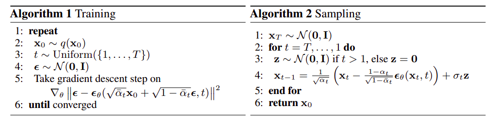
- Let us implement the loss function:
In [9]:
import torch.nn as nn
loss_fn = nn.L1Loss()
def compute_loss(pred_eps_model, x_0, t):
with torch.no_grad():
x_t, true_eps = direct_sampling(x_0, t)
noise_pred = pred_eps_model(x_t, t)
return loss_fn(true_eps, noise_pred)
- And the sampling procedure:
In [10]:
alphas = 1. - betas
alphas_cumprod = torch.cumprod(alphas, axis=0)
sqrt_alphas_cumprod = torch.sqrt(alphas_cumprod)
sqrt_one_minus_alphas_cumprod = torch.sqrt(1. - alphas_cumprod)
sqrt_recip_alphas = torch.sqrt(1.0 / alphas)
alphas_cumprod_prev = F.pad(alphas_cumprod[:-1], (1, 0), value=1.0)
posterior_variance = betas * (1. - alphas_cumprod_prev) / (1. - alphas_cumprod) # β_t
@torch.no_grad()
def p_sample(model, x, t, t_index):
# adjust shapes
betas_t = extract(betas, t, x.shape)
sqrt_one_minus_alphas_cumprod_t = extract(
sqrt_one_minus_alphas_cumprod, t, x.shape
)
sqrt_recip_alphas_t = extract(sqrt_recip_alphas, t, x.shape)
# Use the NN to predict the mean
model_mean = sqrt_recip_alphas_t * (
x - betas_t * model(x, t) / sqrt_one_minus_alphas_cumprod_t)
# Draw the next sample
if t_index == 0:
return model_mean
else:
posterior_variance_t = extract(posterior_variance, t, x.shape) # beta_t
noise = torch.randn_like(x) # z
return model_mean + torch.sqrt(posterior_variance_t) * noise # x_{t-1}
@torch.no_grad()
def p_sample_loop(model, shape):
device = next(model.parameters()).device
# start from pure noise (for each example in the batch)
img = torch.randn(shape, device=device)
imgs = []
for i in tqdm(reversed(range(0, T)), desc='sampling loop time step', total=T):
img = p_sample(model, img, torch.full((shape[0],), i, device=device, dtype=torch.long), i)
imgs.insert(-1,img)
return imgs
@torch.no_grad()
def sample(model, image_size, batch_size=16, channels=1):
return p_sample_loop(model, shape=(batch_size, channels, image_size, image_size))
def sample_plot_image(model):
samples = sample(model, image_size=IMG_SIZE, batch_size=64, channels=1)
imgs_steps = []
num_steps = 10
for i in range(0,len(samples),T//num_steps):
step = samples[i]
last_sample = (step[-1] - step[-1].min())/(step[-1].max()-step[-1].min())
imgs_steps.append(last_sample)
grid_img = torchvision.utils.make_grid(imgs_steps,num_steps)
%matplotlib inline
plt.figure(figsize = (20,10))
plt.imshow(grid_img.permute(1, 2, 0).cpu().numpy(), cmap='gray')
plt.show()
Noise recovery model
- A U-Net like PixelCNN++ backbone:
- Diffusion time $t$ is specified by adding the Transformer sinusoidal position embedding
into each residual block.
In [11]:
import math
class SinusoidalPositionEmbeddings(nn.Module):
def __init__(self, dim):
super().__init__()
self.dim = dim
def forward(self, time):
device = time.device
half_dim = self.dim // 2
embeddings = math.log(10000) / (half_dim - 1)
embeddings = torch.exp(torch.arange(half_dim, device=device) * -embeddings)
embeddings = time[:, None] * embeddings[None, :]
embeddings = torch.cat((embeddings.sin(), embeddings.cos()), dim=-1)
# TODO: Double check the ordering here
return embeddings
- We will implement a simplified version of it here:
In [12]:
from torch import nn
class Block(nn.Module):
def __init__(self, in_ch, out_ch, time_emb_dim, up=False):
super().__init__()
self.time_mlp = nn.Linear(time_emb_dim, out_ch)
if up:
self.conv1 = nn.Conv2d(2*in_ch, out_ch, 3, padding=1)
self.transform = nn.ConvTranspose2d(out_ch, out_ch, 4, 2, 1)
else:
self.conv1 = nn.Conv2d(in_ch, out_ch, 3, padding=1)
self.transform = nn.Conv2d(out_ch, out_ch, 4, 2, 1)
self.conv2 = nn.Conv2d(out_ch, out_ch, 3, padding=1)
self.bnorm1 = nn.BatchNorm2d(out_ch)
self.bnorm2 = nn.BatchNorm2d(out_ch)
self.relu = nn.ReLU()
def forward(self, x, t, ):
# First Conv
h = self.bnorm1(self.relu(self.conv1(x)))
# Time embedding
time_emb = self.relu(self.time_mlp(t))
# Extend last 2 dimensions
time_emb = time_emb[(..., ) + (None, ) * 2]
# Add time channel
h = h + time_emb
# Second Conv
h = self.bnorm2(self.relu(self.conv2(h)))
# Down or Upsample
return self.transform(h)
class SimpleUnet(nn.Module):
"""
A simplified variant of the Unet architecture.
"""
def __init__(self):
super().__init__()
image_channels = 1
down_channels = (64, 128, 256, 512, 1024)
up_channels = (1024, 512, 256, 128, 64)
out_dim = 1
time_emb_dim = 32
# Time embedding
self.time_mlp = nn.Sequential(
SinusoidalPositionEmbeddings(time_emb_dim),
nn.Linear(time_emb_dim, time_emb_dim),
nn.ReLU()
)
# Initial projection
self.conv0 = nn.Conv2d(image_channels, down_channels[0], 3, padding=1)
# Downsample
self.downs = nn.ModuleList([Block(down_channels[i], down_channels[i+1], \
time_emb_dim) \
for i in range(len(down_channels)-1)])
# Upsample
self.ups = nn.ModuleList([Block(up_channels[i], up_channels[i+1], \
time_emb_dim, up=True) \
for i in range(len(up_channels)-1)])
# Edit: Corrected a bug found by Jakub C (see YouTube comment)
self.output = nn.Conv2d(up_channels[-1], out_dim, 1)
def forward(self, x, timestep):
# Embedd time
t = self.time_mlp(timestep)
# Initial conv
x = self.conv0(x)
# Unet
residual_inputs = []
for down in self.downs:
x = down(x, t)
residual_inputs.append(x)
for up in self.ups:
residual_x = residual_inputs.pop()
# Add residual x as additional channels
x = torch.cat((x, residual_x), dim=1)
x = up(x, t)
return self.output(x)
Training the model
In [13]:
from torch.optim import Adam
pred_eps_model = SimpleUnet()
pred_eps_model.to(device)
optimizer = Adam(pred_eps_model.parameters(), lr=0.001)
num_epochs = 10
for epoch in range(num_epochs):
avg_loss = 0
n_batches = 0
for step, batch in enumerate(dataloader):
imgs, _ = batch
imgs = imgs.to(device)
t = torch.randint(0, T, (BATCH_SIZE,), device=device).long().to(device)
optimizer.zero_grad()
loss = compute_loss(pred_eps_model, imgs, t)
loss.backward()
optimizer.step()
avg_loss += loss.item()
n_batches +=1
avg_loss /= n_batches
pred_eps_model.eval()
print(f"Epoch {epoch} | Loss: {avg_loss:.4f} ")
sample_plot_image(pred_eps_model)
pred_eps_model.train()
Epoch 0 | Loss: 0.1065
sampling loop time step: 100%|██████████████████████████████████| 2000/2000 [01:53<00:00, 17.58it/s]

Epoch 1 | Loss: 0.0600
sampling loop time step: 100%|██████████████████████████████████| 2000/2000 [01:53<00:00, 17.58it/s]

Epoch 2 | Loss: 0.0525
sampling loop time step: 100%|██████████████████████████████████| 2000/2000 [01:53<00:00, 17.58it/s]

Epoch 3 | Loss: 0.0492
sampling loop time step: 100%|██████████████████████████████████| 2000/2000 [01:53<00:00, 17.58it/s]

Epoch 4 | Loss: 0.0469
sampling loop time step: 100%|██████████████████████████████████| 2000/2000 [01:53<00:00, 17.58it/s]

Epoch 5 | Loss: 0.0453
sampling loop time step: 100%|██████████████████████████████████| 2000/2000 [01:53<00:00, 17.58it/s]

Epoch 6 | Loss: 0.0445
sampling loop time step: 100%|██████████████████████████████████| 2000/2000 [01:53<00:00, 17.58it/s]

Epoch 7 | Loss: 0.0430
sampling loop time step: 100%|██████████████████████████████████| 2000/2000 [01:53<00:00, 17.58it/s]

Epoch 8 | Loss: 0.0423
sampling loop time step: 100%|██████████████████████████████████| 2000/2000 [01:53<00:00, 17.57it/s]

Epoch 9 | Loss: 0.0420
sampling loop time step: 100%|██████████████████████████████████| 2000/2000 [01:53<00:00, 17.58it/s]

Credits
- This tutorial was written by Mitchell Keren Taraday and Tamir Shor.
- Some of the code parts were adapted from: https://colab.research.google.com/drive/1sjy9odlSSy0RBVgMTgP7s99NXsqglsUL#scrollTo=KOYPSxPf_LL7 and from: https://github.com/FilippoMB/Diffusion_models_tutorial/blob/main/diffusion_from_scratch.ipynb