QR Decomposition¶

• We learned Cholesky decomposition as one approach for solving linear regression.

• Another approach for linear regression uses the QR decomposition.
  This is how the lm() function in R does linear regression.
  This is also how Julia's (and MATLAB's) \ works for rectangular matrices.

We want to understand what is QR and how it is used for solving least squares problem.

Definitions¶

• Assume $\mathbf{X} \in \mathbb{R}^{n \times p}$ has full column rank. Necessarilly $n \ge p$.

• Full QR decomposition:

where
- $\mathbf{Q} \in \mathbb{R}^{n \times n}$, $\mathbf{Q}^T \mathbf{Q} = \mathbf{Q}\mathbf{Q}^T = \mathbf{I}_n$. In other words, $\mathbf{Q}$ is an orthogonal matrix.
- First $p$ columns of $\mathbf{Q}$ form an orthonormal basis of ${\cal R}(\mathbf{X})$ (range or column space of $\mathbf{X}$)
- Last $n-p$ columns of $\mathbf{Q}$ form an orthonormal basis of ${\cal N}(\mathbf{X}^T)$ (null space of $\mathbf{X}^T$) - Recall that $\mathcal{N}(\mathbf{X}^T)=\mathcal{R}(\mathbf{X})^{\perp}$ and $\mathcal{R}(\mathbf{X}) \oplus \mathcal{N}(\mathbf{X}^T) = \mathbb{R}^n$. - $\mathbf{R} \in \mathbb{R}^{n \times p}$ is upper triangular with positive diagonal entries. - The lower $(n-p)\times p$ block of $\mathbf{R}$ is $\mathbf{0}$ (why?).

• Reduced QR decomposition:

where - $\mathbf{Q}_1 \in \mathbb{R}^{n \times p}$, $\mathbf{Q}_1^T \mathbf{Q}_1 = \mathbf{I}_p$. In other words, $\mathbf{Q}_1$ is a partially orthogonal matrix. Note $\mathbf{Q}_1\mathbf{Q}_1^T \neq \mathbf{I}_n$. - $\mathbf{R}_1 \in \mathbb{R}^{p \times p}$ is an upper triangular matrix with positive diagonal entries.

• Given QR decomposition $\mathbf{X} = \mathbf{Q} \mathbf{R}$, $$ \mathbf{X}^T \mathbf{X} = \mathbf{R}^T \mathbf{Q}^T \mathbf{Q} \mathbf{R} = \mathbf{R}^T \mathbf{R} = \mathbf{R}_1^T \mathbf{R}_1. $$
  • Once we have a (reduced) QR decomposition of $\mathbf{X}$, we automatically have the Cholesky decomposition of the Gram matrix $\mathbf{X}^T \mathbf{X}$.

Application: least squares¶

• Normal equation

is equivalently written with reduced QR as $$ \mathbf{R}_1^T\mathbf{R}_1\beta = \mathbf{R}_1^T\mathbf{Q}_1^T\mathbf{y} $$

• Since $\mathbf{R}_1$ is invertible, we only need to solve the triangluar system

Multiplication $\mathbf{Q}_1^T \mathbf{y}$ is done implicitly (see below).

• This method is numerically more stable than directly solving the normal equation, since $\kappa(\mathbf{X}^T\mathbf{X}) = \kappa(\mathbf{X})^2$!

• In case we need standard errors, compute inverse of $\mathbf{R}_1^T \mathbf{R}_1$. This involves triangular solves.

Gram-Schmidt procedure¶

• Wait! Does $\mathbf{X}$ always have a QR decomposition?
  • Yes. It is equivalent to the Gram-Schmidt procedure for basis orthonormalization.

Jørgen Pedersen Gram, 1850-1916

Erhard Schmidt, 1876-1959

• Assume $\mathbf{X} = [\mathbf{x}_1 | \dotsb | \mathbf{x}_p] \in \mathbb{R}^{n \times p}$ has full column rank. That is, $\mathbf{x}_1,\ldots,\mathbf{x}_p$ are linearly independent.

• Gram-Schmidt (GS) procedure produces nested orthonormal basis vectors $\{\mathbf{q}_1, \dotsc, \mathbf{q}_p\}$ that spans $\mathcal{R}(\mathbf{X})$, i.e.,

and $\langle \mathbf{q}_i, \mathbf{q}_j \rangle = \delta_{ij}$.

• The algorithm: 0. Initialize $\mathbf{q}_1 = \mathbf{x}_1 / \|\mathbf{x}_1\|_2$ 0. For $k=2, \ldots, p$,

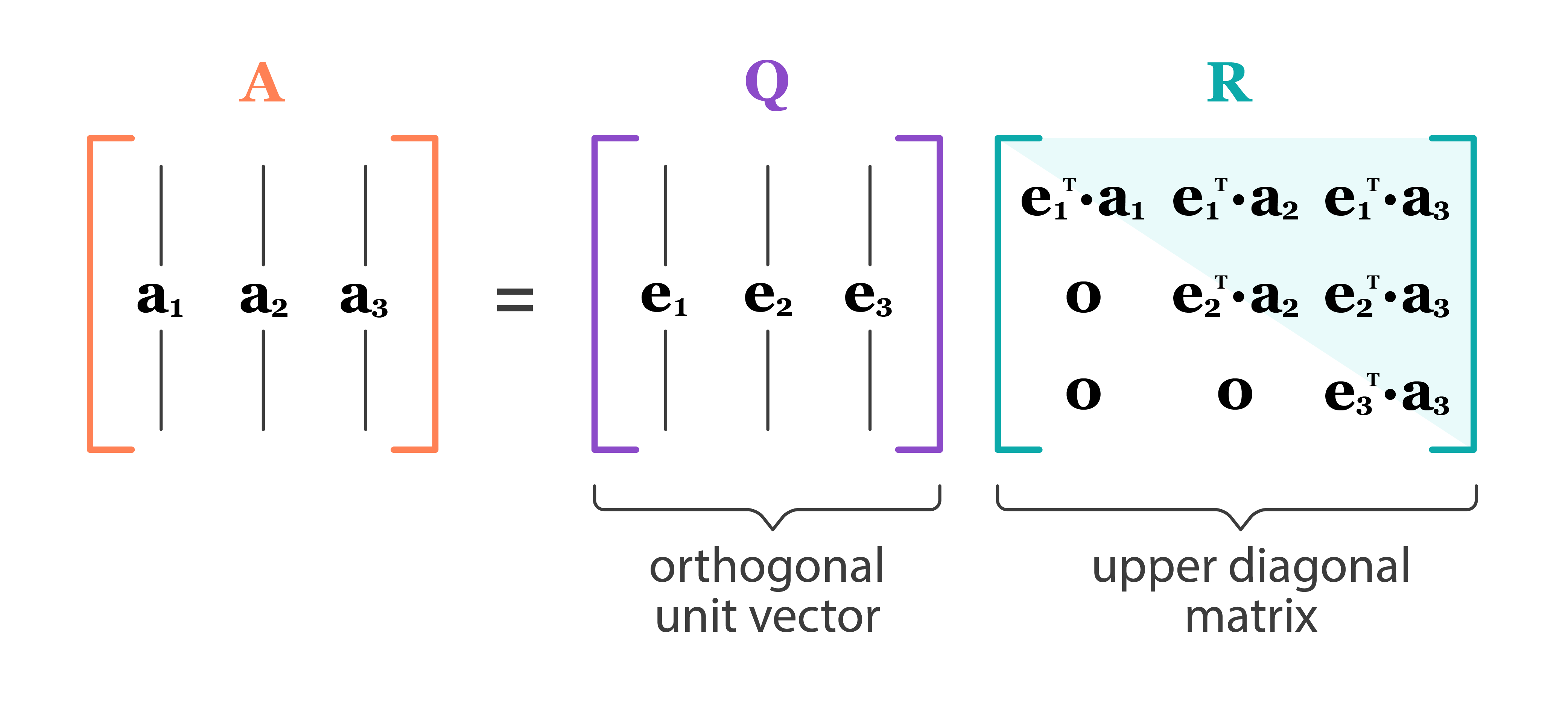
GS conducts reduced QR¶

• $\mathbf{Q} = [\mathbf{q}_1 | \dotsb | \mathbf{q}_p]$. Obviously $\mathbf{Q}^T \mathbf{Q} = \mathbf{I}_p$.

• Where is $\mathbf{R}$?

  • Let $r_{jk} = \langle \mathbf{q}_j, \mathbf{x}_k \rangle$ for $j < k$, and $r_{kk} = \|\mathbf{v}_k\|_2$.
  • Re-write the above expression:

    or

- If we let $r_{jk} = 0$ for $j > k$, then $\mathbf{R}=(r_{jk})$ is upper triangular and $$ \mathbf{X} = \mathbf{Q}\mathbf{R} . $$

Source: https://dsc-spidal.github.io/harp/docs/harpdaal/algorithms/

Classical Gram-Schmidt¶

• CGS is unstable (we lose orthogonality due to roundoff errors) when columns of $\mathbf{X}$ are almost collinear.

• Q is hardly orthogonal.
• Where exactly does the problem occur? (HW)

Modified Gram-Schmidt¶

• The algorithm: 0. Initialize $\mathbf{q}_1 = \mathbf{x}_1 / \|\mathbf{x}_1\|_2$ 0. For $k=2, \ldots, p$,

• $\mathbf{X}$ is overwritten by $\mathbf{Q}$ and $\mathbf{R}$ is stored in a separate array.

• So MGS is more stable than CGS. However, even MGS is not completely immune to instability.

• Q is hardly orthogonal.
• Where exactly the problem occurs? (HW)

• Computational cost of CGS and MGS is $\sum_{k=1}^p 4n(k-1) \approx 2np^2$.

• There are 3 algorithms to compute QR: (modified) Gram-Schmidt, Householder transform, (fast) Givens transform.

  In particular, the Householder transform for QR is implemented in LAPACK and thus used in R and Julia.

QR by Householder transform¶

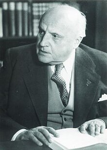
Alston Scott Householder (1904-1993)

• This is the algorithm for solving linear regression in R.

• Assume again $\mathbf{X} = [\mathbf{x}_1 | \dotsb | \mathbf{x}_p] \in \mathbb{R}^{n \times p}$ has full column rank.

• Gram-Schmidt can be understood as:

where $\mathbf{R}_j$ are a sequence of upper triangular matrices.

• Householder QR does

where $\mathbf{H}_j \in \mathbf{R}^{n \times n}$ are a sequence of Householder transformation matrices.

It yields the **full QR** where $\mathbf{Q} = \mathbf{H}_1 \cdots \mathbf{H}_p \in \mathbb{R}^{n \times n}$. Recall that CGS/MGS only produces the **reduced QR** decomposition.

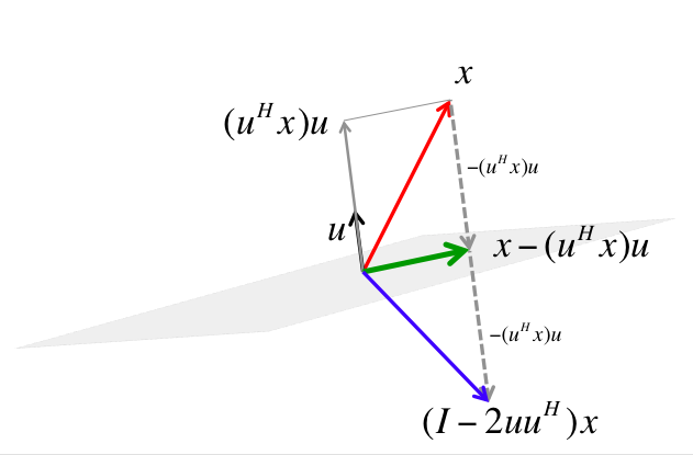
• For arbitrary $\mathbf{v}, \mathbf{w} \in \mathbb{R}^{n}$ with $\|\mathbf{v}\|_2 = \|\mathbf{w}\|_2$, we can construct a Householder matrix (or Householder reflector)

that transforms $\mathbf{v}$ to $\mathbf{w}$: $$ \mathbf{H} \mathbf{v} = \mathbf{w}. $$ $\mathbf{H}$ is symmetric and orthogonal. Calculation of Householder vector $\mathbf{u}$ costs $4n$ flops for general $\mathbf{u}$ and $\mathbf{w}$.

Source: https://www.cs.utexas.edu/users/flame/laff/alaff-beta/images/Chapter03/reflector.png

• Now choose $\mathbf{H}_1$ so that

That is, $\mathbf{v} = \mathbf{x}_1$ and $\mathbf{w} = \|\mathbf{x}_1\|_2\mathbf{e}_1$.

• Left-multiplying $\mathbf{H}_1$ zeros out the first column of $\mathbf{X}$ below (1, 1).

• Take $\mathbf{H}_2$ to zero the second column below diagonal:

• In general, choose the $j$-th Householder transform $\mathbf{H}_j = \mathbf{I}_n - 2 \mathbf{u}_j \mathbf{u}_j^T$, where

to zero the $j$-th column below diagonal. $\mathbf{H}_j$ takes the form $$ \mathbf{H}_j = \begin{bmatrix} \mathbf{I}_{j-1} & \\ & \mathbf{I}_{n-j+1} - 2 {\tilde u}_j {\tilde u}_j^T \end{bmatrix} = \begin{bmatrix} \mathbf{I}_{j-1} & \\ & {\tilde H}_{j} \end{bmatrix}. $$

• Applying a Householder transform $\mathbf{H} = \mathbf{I} - 2 \mathbf{u} \mathbf{u}^T$ to a matrix $\mathbf{X} \in \mathbb{R}^{n \times p}$

costs $4np$ flops. Householder updates never entails explicit formation of the Householder matrices.

• Note applying ${\tilde H}_j$ to $\mathbf{X}$ only needs $4(n-j+1)(p-j+1)$ flops.

Algorithm¶

for j=1:p
    u = House!(X[j:n, j])
    for i=j:p
        X[j:n, j:p] .-= 2u*(u'X[j:n, j:p])
    end
end

• The process is done in place. Upper triangular part of $\mathbf{X}$ is overwritten by $\mathbf{R}_1$ and the essential Householder vectors ($\tilde u_{j1}$ is normalized to 1) are stored in $\mathbf{X}[j:n,j]$.

• At $j$-th stage 0. computing the Householder vector ${\tilde u}_j$ costs $3(n-j+1)$ flops 0. applying the Householder transform ${\tilde H}_j$ to the $\mathbf{X}[j:n, j:p]$ block costs $4(n-j+1)(p-j+1)$ flops

• In total we need $\sum_{j=1}^p [3(n-j+1) + 4(n-j+1)(p-j+1)] \approx 2np^2 - \frac 23 p^3$ flops.

• Where is $\mathbf{Q}$?

  • $\mathbf{Q} = \mathbf{H}_1 \cdots \mathbf{H}_p$. In some applications, it's necessary to form the orthogonal matrix $\mathbf{Q}$.

  Accumulating $\mathbf{Q}$ costs another $2np^2 - \frac 23 p^3$ flops.

• When computing $\mathbf{Q}^T \mathbf{v}$ or $\mathbf{Q} \mathbf{v}$ as in some applications (e.g., solve linear equation using QR), no need to form $\mathbf{Q}$. Simply apply Householder transforms successively to the vector $\mathbf{v}$. (HW)

• Computational cost of Householder QR for linear regression: $2n p^2 - \frac 23 p^3$ (regression coefficients and $\hat \sigma^2$) or more (fitted values, s.e., ...).

Householder QR with column pivoting¶

Consider rank deficient $\mathbf{X}$.

• At the $j$-th stage, swap the column X[:, j] with X[:, k] where k is the column number in X[j:n,j:p] with maximum $\ell_2$ norm to be the pivot column. If the maximum $\ell_2$ norm is 0, it stops, ending with

where $\mathbf{P} \in \mathbb{R}^{p \times p}$ is a permutation matrix and $r$ is the rank of $\mathbf{X}$. QR with column pivoting is rank revealing.

Implementation¶

• Julia functions: qr, qrfact!, or call LAPACK wrapper functions geqrf! and geqp3!

• R function: qr. Wraps LAPACK routine dgeqp3 (with LAPACK=TRUE; default uses LINPACK, an ancient version of LAPACK).

QR by Givens rotation¶

• Householder transform $\mathbf{H}_j$ introduces batch of zeros into a vector.

• Givens transform (aka Givens rotation, Jacobi rotation, plane rotation) selectively zeros one element of a vector.

• Overall QR by Givens rotation is less efficient than the Householder method, but is better suited for matrices with structured patterns of nonzero elements.

• Givens/Jacobi rotations:

where $c = \cos(\theta)$ and $s = \sin(\theta)$. $\mathbf{G}(i,k,\theta)$ is orthogonal.

• Pre-multiplication by $\mathbf{G}(i,k,\theta)^T$ rotates counterclockwise $\theta$ radians in the $(i,k)$ coordinate plane. If $\mathbf{x} \in \mathbb{R}^n$ and $\mathbf{y} = \mathbf{G}(i,k,\theta)^T \mathbf{x}$, then

Apparently if we choose $\tan(\theta) = -x_k / x_i$, or equivalently, $$ \begin{eqnarray*} c = \frac{x_i}{\sqrt{x_i^2 + x_k^2}}, \quad s = \frac{-x_k}{\sqrt{x_i^2 + x_k^2}}, \end{eqnarray*} $$ then $y_k=0$.

• Pre-applying Givens transform $\mathbf{G}(i,k,\theta)^T \in \mathbb{R}^{n \times n}$ to a matrix $\mathbf{A} \in \mathbb{R}^{n \times m}$ only effects two rows of $\mathbf{

A}$: $$ \mathbf{A}([i, k], :) \gets \begin{bmatrix} c & s \\ -s & c \end{bmatrix}^T \mathbf{A}([i, k], :), $$ costing $6m$ flops.

• Post-applying Givens transform $\mathbf{G}(i,k,\theta) \in \mathbb{R}^{m \times m}$ to a matrix $\mathbf{A} \in \mathbb{R}^{n \times m}$ only effects two columns of $\mathbf{A}$:

costing $6n$ flops.

• QR by Givens: $\mathbf{G}_t^T \cdots \mathbf{G}_1^T \mathbf{X} = \begin{bmatrix} \mathbf{R}_1 \\ \mathbf{0} \end{bmatrix}$.

• Zeros in $\mathbf{X}$ can also be introduced row-by-row.

• If $\mathbf{X} \in \mathbb{R}^{n \times p}$, the total cost is $3np^2 - p^3$ flops and $O(np)$ square roots.

• Note each Givens transform can be summarized by a single number, which is stored in the zeroed entry of $\mathbf{X}$.

Applications¶

Linear regression¶

• QR decomposition of $\mathbf{X}$: $2np^2 - \frac 23 p^3$ flops.

• Solve $\mathbf{R}^T \mathbf{R} \beta = \mathbf{R}^T \mathbf{Q}^T \mathbf{y}$ for $\beta$.

• If $\mathbf{X}$ is full rank, then $\mathbf{R}$ is invertible, so we only need to solve the triangular system

Multiplication $\mathbf{Q}^T \mathbf{y}$ is done implicitly.

• If need standard errors, compute inverse of $\mathbf{R}^T \mathbf{R}$. This involves triangular solves.

Further reading¶

• Section II.5.3 of Computational Statistics by James Gentle (2010).

• Chapter 5 of Matrix Computation by Gene Golub and Charles Van Loan (2013).

Acknowledgment¶

Many parts of this lecture note is based on Dr. Hua Zhou's 2019 Spring Statistical Computing course notes available at http://hua-zhou.github.io/teaching/biostatm280-2019spring/index.html.