QR Decomposition¶

• We learned Cholesky decomposition as one approach for solving linear regression.

• Another approach for linear regression uses the QR decomposition.
  This is how the lm() function in R does linear regression.
  This is also how Julia's (and MATLAB's) \ works for rectangular matrices.

We want to understand what is QR and how it is used for solving least squares problem.

Definitions¶

• Assume $\mathbf{X} \in \mathbb{R}^{n \times p}$ has full column rank. Necessarilly $n \ge p$.

• Full QR decomposition:

- $\mathbf{Q} \in \mathbb{R}^{n \times n}$, $\mathbf{Q}^T \mathbf{Q} = \mathbf{Q}\mathbf{Q}^T = \mathbf{I}_n$. In other words, $\mathbf{Q}$ is an orthogonal matrix.  
    - First $p$ columns of $\mathbf{Q}$ form an orthonormal basis of ${\cal R}(\mathbf{X})$ (**range** or column space of $\mathbf{X}$)      
    - Last $n-p$ columns of $\mathbf{Q}$ form an orthonormal basis of ${\cal N}(\mathbf{X}^T)$ (**null space** of $\mathbf{X}^T$)
- Recall that $\mathcal{N}(\mathbf{X}^T)=\mathcal{R}(\mathbf{X})^{\perp}$ and $\mathcal{R}(\mathbf{X}) \oplus \mathcal{N}(\mathbf{X}^T) = \mathbb{R}^n$.
- $\mathbf{R} \in \mathbb{R}^{n \times p}$  is upper triangular with positive diagonal entries. 
    - The lower $(n-p)\times p$ block of $\mathbf{R}$ is $\mathbf{0}$ (why?).

• Reduced QR decomposition:

where - $\mathbf{Q}_1 \in \mathbb{R}^{n \times p}$, $\mathbf{Q}_1^T \mathbf{Q}_1 = \mathbf{I}_p$. In other words, $\mathbf{Q}_1$ is a partially orthogonal matrix. Note $\mathbf{Q}_1\mathbf{Q}_1^T \neq \mathbf{I}_n$. - $\mathbf{R}_1 \in \mathbb{R}^{p \times p}$ is an upper triangular matrix with positive diagonal entries.

• Given QR decomposition $\mathbf{X} = \mathbf{Q} \mathbf{R}$, $$ \mathbf{X}^T \mathbf{X} = \mathbf{R}^T \mathbf{Q}^T \mathbf{Q} \mathbf{R} = \mathbf{R}^T \mathbf{R} = \mathbf{R}_1^T \mathbf{R}_1. $$
  • Once we have a (reduced) QR decomposition of $\mathbf{X}$, we automatically have the Cholesky decomposition of the Gram matrix $\mathbf{X}^T \mathbf{X}$.

Application: least squares¶

• Normal equation

is equivalently written with reduced QR as $$ \mathbf{R}_1^T\mathbf{R}_1\beta = \mathbf{R}_1^T\mathbf{Q}_1^T\mathbf{y} $$

• $\mathbf{R}_1$ is invertible: we only need to solve the triangluar system

Multiplication $\mathbf{Q}_1^T \mathbf{y}$ is done implicitly (see below).

• This method is numerically more stable than directly solving the normal equation, since $\kappa(\mathbf{X}^T\mathbf{X}) = \kappa(\mathbf{X})^2$!

• In case we need standard errors, compute inverse of $\mathbf{R}_1^T \mathbf{R}_1$. This involves triangular solves.

Gram-Schmidt procedure¶

• Wait! Does $\mathbf{X}$ always have a QR decomposition?
  • Yes. It is equivalent to the Gram-Schmidt procedure for basis orthonormalization.

:::: {.columns}

::: {.column width="50%"}

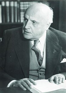
Jørgen Pedersen Gram, 1850-1916 :::

::: {.column width="50%"}

Erhard Schmidt, 1876-1959 :::

::::

• Assume $\mathbf{X} = [\mathbf{x}_1 | \dotsb | \mathbf{x}_p] \in \mathbb{R}^{n \times p}$ has full column rank. That is, $\mathbf{x}_1,\ldots,\mathbf{x}_p$ are linearly independent.

• Gram-Schmidt (GS) procedure produces nested orthonormal basis vectors $\{\mathbf{q}_1, \dotsc, \mathbf{q}_p\}$ that spans $\mathcal{R}(\mathbf{X})$, i.e.,

and $\langle \mathbf{q}_i, \mathbf{q}_j \rangle = \delta_{ij}$.

• The algorithm: 0. Initialize $\mathbf{q}_1 = \mathbf{x}_1 / \|\mathbf{x}_1\|_2$ 0. For $k=2, \ldots, p$,

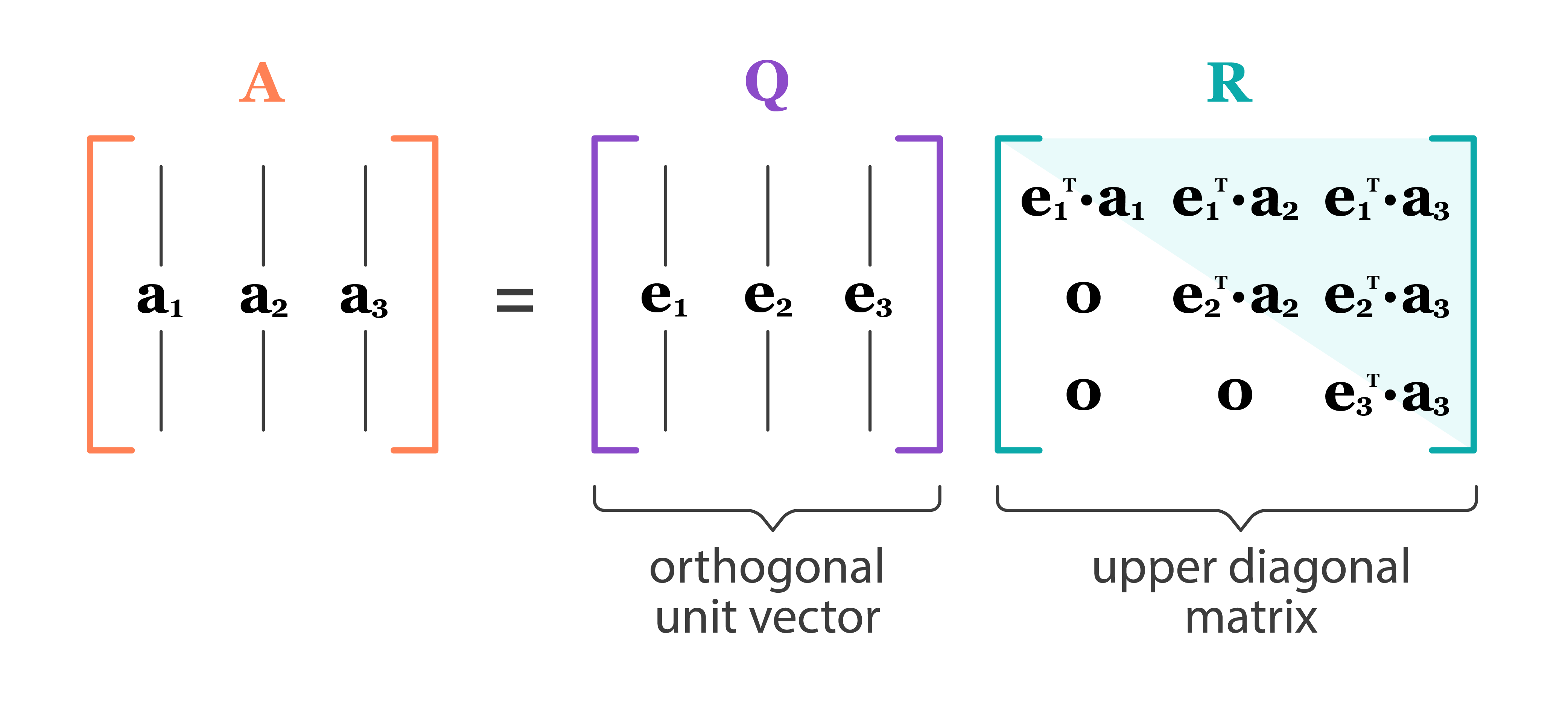
GS conducts reduced QR¶

• $\mathbf{Q} = [\mathbf{q}_1 | \dotsb | \mathbf{q}_p]$. Obviously $\mathbf{Q}^T \mathbf{Q} = \mathbf{I}_p$.

• Where is $\mathbf{R}$?

  • Let $r_{jk} = \langle \mathbf{q}_j, \mathbf{x}_k \rangle$ for $j < k$, and $r_{kk} = \|\mathbf{v}_k\|_2$.
  • Re-write the above expression:

    or

- If we let $r_{jk} = 0$ for $j > k$, then $\mathbf{R}=(r_{jk})$ is upper triangular and $$ \mathbf{X} = \mathbf{Q}\mathbf{R} . $$

{background-color="white"}¶

{width=800}

Classical Gram-Schmidt¶

• CGS is unstable (we lose orthogonality due to roundoff errors) when columns of $\mathbf{X}$ are almost collinear.

• Q is hardly orthogonal.
• Where exactly does the problem occur? (HW)

Modified Gram-Schmidt¶

• The algorithm: 0. Initialize $\mathbf{q}_1 = \mathbf{x}_1 / \|\mathbf{x}_1\|_2$ 0. For $k=2, \ldots, p$,

• $\mathbf{X}$ is overwritten by $\mathbf{Q}$ and $\mathbf{R}$ is stored in a separate array.

• So MGS is more stable than CGS. However, even MGS is not completely immune to instability.

• Q is hardly orthogonal.
• Where exactly the problem occurs? (HW)

• Computational cost of CGS and MGS is $\sum_{k=1}^p 4n(k-1) \approx 2np^2$.

• There are 3 algorithms to compute QR: (modified) Gram-Schmidt, Householder transform, (fast) Givens transform.

  In particular, the Householder transform for QR is implemented in LAPACK and thus used in R and Julia.

QR by Householder transform¶

{width=200}

• This is the algorithm for solving linear regression in R.

• Assume again $\mathbf{X} = [\mathbf{x}_1 | \dotsb | \mathbf{x}_p] \in \mathbb{R}^{n \times p}$ has full column rank.

• Gram-Schmidt can be understood as:

where $\mathbf{R}_j$ are a sequence of upper triangular matrices.

• Householder QR does

where $\mathbf{H}_j \in \mathbf{R}^{n \times n}$ are a sequence of Householder transformation matrices.

It yields the **full QR** where $\mathbf{Q} = \mathbf{H}_1 \cdots \mathbf{H}_p \in \mathbb{R}^{n \times n}$. Recall that CGS/MGS only produces the **reduced QR** decomposition.

Householder transformation¶

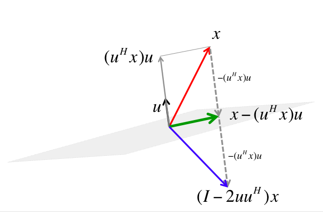
• For arbitrary $\mathbf{v}, \mathbf{w} \in \mathbb{R}^{n}$ with $\|\mathbf{v}\|_2 = \|\mathbf{w}\|_2$, we can construct a Householder matrix (or Householder reflector)

that transforms $\mathbf{v}$ to $\mathbf{w}$: $$ \mathbf{H} \mathbf{v} = \mathbf{w}. $$ $\mathbf{H}$ is symmetric and orthogonal. Calculation of Householder vector $\mathbf{u}$ costs $4n$ flops for general $\mathbf{u}$ and $\mathbf{w}$.

{width=400}

• Now choose $\mathbf{H}_1$ so that

That is, $\mathbf{x} = \mathbf{x}_1$ and $\mathbf{w} = \pm\|\mathbf{x}_1\|_2\mathbf{e}_1$.

• Left-multiplying $\mathbf{H}_1$ zeros out the first column of $\mathbf{X}$ below (1, 1).

• Take $\mathbf{H}_2$ to zero the second column below diagonal:

• In general, choose the $j$-th Householder transform $\mathbf{H}_j = \mathbf{I}_n - 2 \mathbf{u}_j \mathbf{u}_j^T$, where

to zero the $j$-th column below diagonal. $\mathbf{H}_j$ takes the form $$ \mathbf{H}_j = \begin{bmatrix} \mathbf{I}_{j-1} & \\ & \mathbf{I}_{n-j+1} - 2 {\tilde u}_j {\tilde u}_j^T \end{bmatrix} = \begin{bmatrix} \mathbf{I}_{j-1} & \\ & {\tilde H}_{j} \end{bmatrix}. $$

• Applying a Householder transform $\mathbf{H} = \mathbf{I} - 2 \mathbf{u} \mathbf{u}^T$ to a matrix $\mathbf{X} \in \mathbb{R}^{n \times p}$

costs $4np$ flops. Householder updates never entails explicit formation of the Householder matrices.

• Note applying ${\tilde H}_j$ to $\mathbf{X}$ only needs $4(n-j+1)(p-j+1)$ flops.

Algorithm¶

for j=1:p
    u = House!(X[j:n, j])
    for i=j:p
        X[j:n, j:p] .-= 2u*(u'X[j:n, j:p])
    end
end

• The process is done in place. Upper triangular part of $\mathbf{X}$ is overwritten by $\mathbf{R}_1$ and the essential Householder vectors ($\tilde u_{j1}$ is normalized to 1) are stored in $\mathbf{X}[j:n,j]$.

  • Can ensure $u_{j1} \neq 0$ by a clever choice of the sign in determining vector $\mathbf{w}$ above (HW).

• At the $j$-th stage

  1. computing the Householder vector ${\tilde u}_j$ costs $3(n-j+1)$ flops
  2. applying the Householder transform ${\tilde H}_j$ to the $\mathbf{X}[j:n, j:p]$ block costs $4(n-j+1)(p-j+1)$ flops

• In total we need $\sum_{j=1}^p [3(n-j+1) + 4(n-j+1)(p-j+1)] \approx 2np^2 - \frac 23 p^3$ flops.

• Where is $\mathbf{Q}$?

  • $\mathbf{Q} = \mathbf{H}_1 \cdots \mathbf{H}_p$. In some applications, it's necessary to form the orthogonal matrix $\mathbf{Q}$.

  Accumulating $\mathbf{Q}$ costs another $2np^2 - \frac 23 p^3$ flops.

• When computing $\mathbf{Q}^T \mathbf{v}$ or $\mathbf{Q} \mathbf{v}$ as in some applications (e.g., solve linear equation using QR), no need to form $\mathbf{Q}$. Simply apply Householder transforms successively to the vector $\mathbf{v}$. (HW)

• Computational cost of Householder QR for linear regression: $2n p^2 - \frac 23 p^3$ (regression coefficients and $\hat \sigma^2$) or more (fitted values, s.e., ...).

Householder QR with column pivoting¶

Consider rank deficient $\mathbf{X}$.

• At the $j$-th stage, swap the column X[:, j] with X[:, k] where k is the column number in X[j:n,j:p] with maximum $\ell_2$ norm to be the pivot column. If the maximum $\ell_2$ norm is 0, it stops, ending with

where $\mathbf{P} \in \mathbb{R}^{p \times p}$ is a permutation matrix and $r$ is the rank of $\mathbf{X}$. QR with column pivoting is rank revealing.

Implementation¶

• Julia functions: qr, qrfact!, or call LAPACK wrapper functions geqrf! and geqp3!

• R function: qr. Wraps LAPACK routine dgeqp3 (with LAPACK=TRUE; default uses LINPACK, an ancient version of LAPACK).

QR by Givens rotation¶

• Householder transform $\mathbf{H}_j$ introduces batch of zeros into a vector.

• Givens transform (aka Givens rotation, Jacobi rotation, plane rotation) selectively zeros one element of a vector.

• Overall QR by Givens rotation is less efficient than the Householder method, but is better suited for matrices with structured patterns of nonzero elements.

• Givens/Jacobi rotations:

where $c = \cos(\theta)$ and $s = \sin(\theta)$. $\mathbf{G}(i,k,\theta)$ is orthogonal.

• Pre-multiplication by $\mathbf{G}(i,k,\theta)^T$ rotates counterclockwise $\theta$ radians in the $(i,k)$ coordinate plane. If $\mathbf{x} \in \mathbb{R}^n$ and $\mathbf{y} = \mathbf{G}(i,k,\theta)^T \mathbf{x}$, then

Apparently if we choose $\tan(\theta) = -x_k / x_i$, or equivalently, $$ \small \begin{eqnarray*} c = \frac{x_i}{\sqrt{x_i^2 + x_k^2}}, \quad s = \frac{-x_k}{\sqrt{x_i^2 + x_k^2}}, \end{eqnarray*} $$ then $y_k=0$.

• Pre-applying Givens transform $\mathbf{G}(i,k,\theta)^T \in \mathbb{R}^{n \times n}$ to a matrix $\mathbf{A} \in \mathbb{R}^{n \times m}$ only effects two rows of $\mathbf{

A}$: $$ \mathbf{A}([i, k], :) \gets \begin{bmatrix} c & s \\ -s & c \end{bmatrix}^T \mathbf{A}([i, k], :), $$ costing $6m$ flops.

• Post-applying Givens transform $\mathbf{G}(i,k,\theta) \in \mathbb{R}^{m \times m}$ to a matrix $\mathbf{A} \in \mathbb{R}^{n \times m}$ only effects two columns of $\mathbf{A}$:

costing $6n$ flops.

• QR by Givens: $\mathbf{G}_t^T \cdots \mathbf{G}_1^T \mathbf{X} = \begin{bmatrix} \mathbf{R}_1 \\ \mathbf{0} \end{bmatrix}$.

{width=600}

• Zeros in $\mathbf{X}$ can also be introduced row-by-row.

• If $\mathbf{X} \in \mathbb{R}^{n \times p}$, the total cost is $3np^2 - p^3$ flops and $O(np)$ square roots.

• Note each Givens transform can be summarized by a single number, which is stored in the zeroed entry of $\mathbf{X}$.

Applications: linear regression¶

• QR decomposition of $\mathbf{X}$: $2np^2 - \frac 23 p^3$ flops.

• Solve $\mathbf{R}^T \mathbf{R} \beta = \mathbf{R}^T \mathbf{Q}^T \mathbf{y}$ for $\beta$.

• If $\mathbf{X}$ is full rank, then $\mathbf{R}$ is invertible, so we only need to solve the triangular system

Multiplication $\mathbf{Q}^T \mathbf{y}$ is done implicitly.

• If need standard errors, compute inverse of $\mathbf{R}^T \mathbf{R}$. This involves triangular solves.

Further reading¶

• Section II.5.3 of Computational Statistics by James Gentle (2010).

• Chapter 5 of Matrix Computation by Gene Golub and Charles Van Loan (2013).