GATK Tutorial :: Germline SNPs & Indels :: Worksheet
March 2019
| . | . |
|---|---|
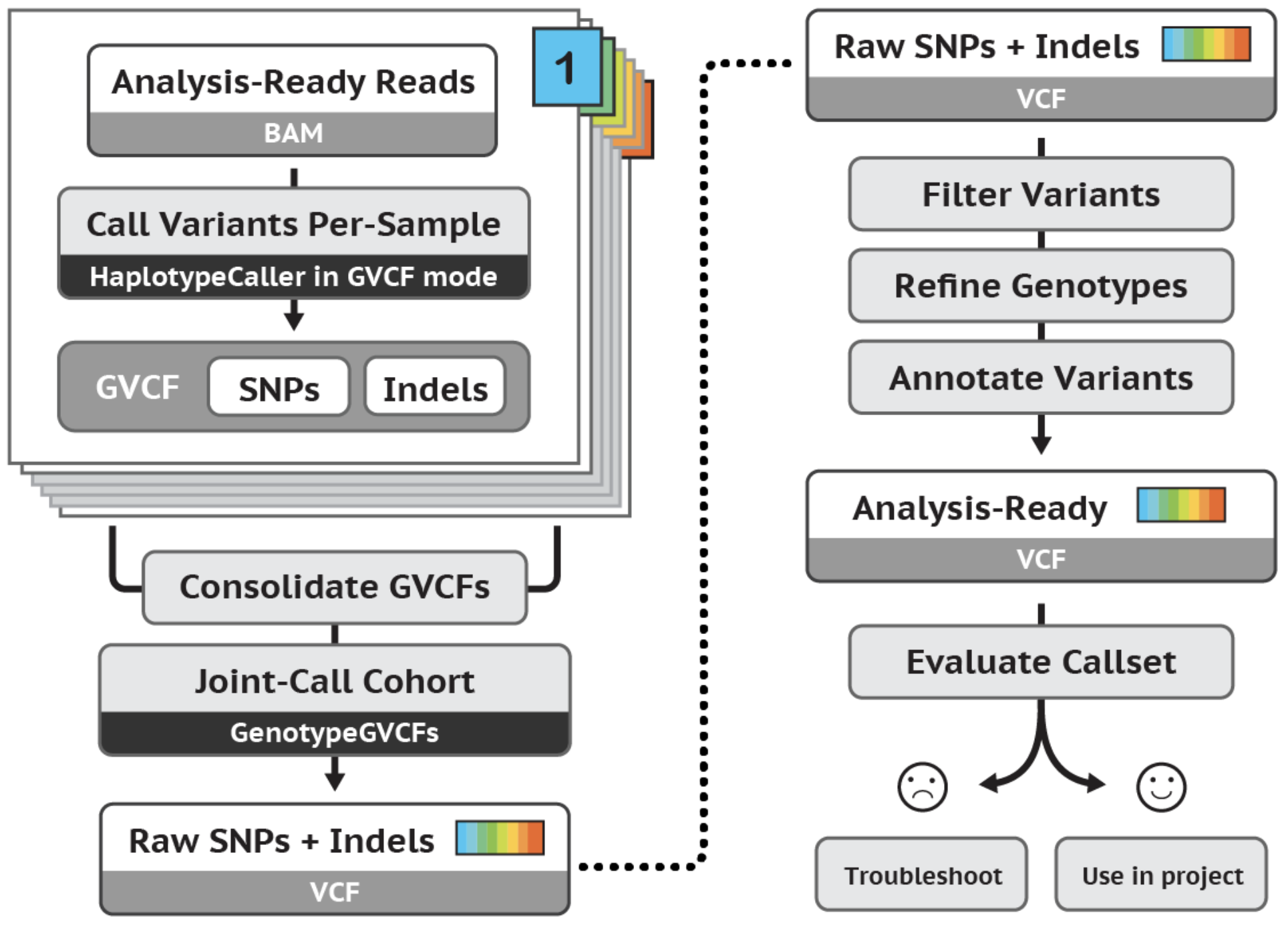 |
The tutorial demonstrates an effective workflow for joint calling germline SNPs and indels in cohorts of multiple samples. The workflow applies to whole genome or exome data. Specifically, the tutorial uses a trio of WG sample snippets to demonstrate HaplotypeCaller's GVCF workflow for joint variant analysis. We use a GenomicsDB database structure, perform a genotype refinement based on family pedigree, and evaluate the effects of refinement. |
The tutorial was last tested with the broadinstitute/gatk:4.1.0.0 docker and IGV v2.4.13.
Table of Contents
- HAPLOTYPECALLER BASICS 1.1 Call variants with HaplotypeCaller in default VCF mode 1.2 View realigned reads and assembled haplotypes
- GVCF WORKFLOW 2.1 Run HaplotypeCaller on a single bam file in GVCF mode 2.2 Consolidate GVCFs using GenomicsDBImport 2.3 Run joint genotyping on the trio to generate the VCF
- GENOTYPE REFINEMENT 3.1 Refine the genotype calls with CalculateGenotypePosteriors 3.2 Compare changes with CollectVariantCallingMetrics
First, make sure the notebook is using a Python 3 kernel in the top right corner.
A kernel is a computational engine that executes the code in the notebook. We can execute GATK commands using Python Magic (!).
How to run this notebook:
- Click to select a gray cell and then pressing SHIFT+ENTER to run the cell.
- Write results to
/home/jupyter-user/2-germline-vd/sandbox/. To access the directory, click on the upper-left jupyter icon. - Your output directory will be synced with your workspace bucket in order to view the results using IGV
# Create your sandbox directory
! mkdir -p /home/jupyter-user/2-germline-vd/sandbox/

# Set you workspace bucket name. **Replace with your bucket**
%env BUCKET=fc-ea3b695a-7c46-4996-b1ef-7112c1ce5b27

# copy files from your notebook sandbox to your workspace bucket sandbox
! gsutil cp -a public-read /home/jupyter-user/2-germline-vd/sandbox/* gs://$BUCKET/sandbox
Enable reading Google bucket data
# Check if data is accessible. The command should list several gs:// URLs.
! gsutil ls gs://gatk-tutorials/workshop_1903/2-germline/
# If you do not see gs:// URLs listed above, run this cell to install Google Cloud Storage.
# Afterwards, restart the kernel with Kernel > Restart.
! pip install google-cloud-storage
Download Data to the Notebook
Some tools are not able to read directly from a googe bucket, we download their files locally.
! mkdir /home/jupyter-user/2-germline-vd/ref
! mkdir /home/jupyter-user/2-germline-vd/resources
! gsutil cp gs://gatk-tutorials/workshop_1903/2-germline/ref/* /home/jupyter-user/2-germline-vd/ref
! gsutil cp gs://gatk-tutorials/workshop_1903/2-germline/trio.ped /home/jupyter-user/2-germline-vd/
! gsutil cp gs://gatk-tutorials/workshop_1903/2-germline/resources/* /home/jupyter-user/2-germline-vd/resources/
Setup IGV
- Download IGV to your local machine if you haven't already done so.
- Follow the instructions to setup your google account with IGV using this document: Browse_Genomic_Data. This allows you to access data from your workspace bucket.
Call variants with HaplotypeCaller in default VCF mode
In this first step we run HaplotypeCaller in its simplest form on a single sample to get familiar with its operation and to learn some useful tips and tricks.
! gatk HaplotypeCaller \
    -R gs://gatk-tutorials/workshop_1903/2-germline/ref/ref.fasta \
    -I gs://gatk-tutorials/workshop_1903/2-germline/bams/mother.bam \
    -O /home/jupyter-user/2-germline-vd/sandbox/motherHC.vcf \
    -L 20:10,000,000-10,200,000
# copy files from your notebook sandbox to your workspace bucket sandbox
! gsutil cp -a public-read /home/jupyter-user/2-germline-vd/sandbox/* gs://$BUCKET/sandbox
! echo gs://$BUCKET/sandbox/motherHC.vcf
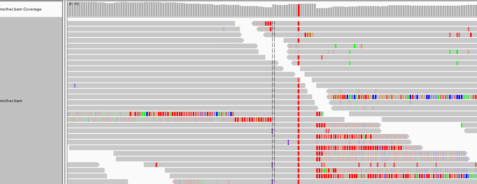
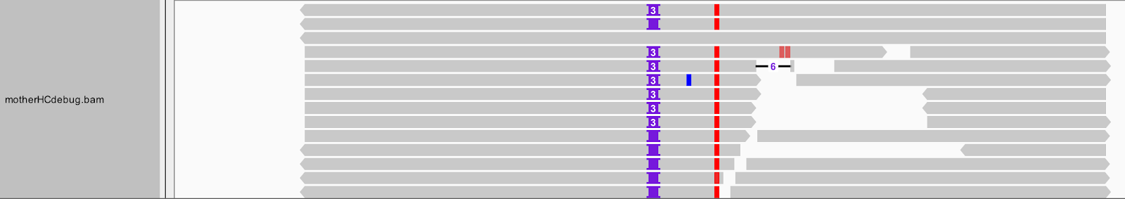
Load the input BAM file as well as the output VCF (sandbox/motherHC.vcf) in IGV and go to the coordinates 20:10,002,294-10,002,623. Be sure the genome is set to b37.
We see that HaplotypeCaller called a homozygous variant insertion of three T bases. How is this possible when so few reads seem to support an insertion at this position?
| Tool Tip | . |
|---|---|
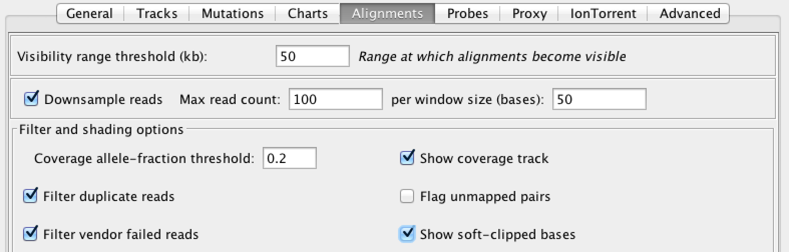 |
When you encounter indel-related weirdness, turn on the display of soft-clips, which IGV turns off by default. Go to View > Preferences > Alignments and select “Show soft-clipped bases” |
With soft clip display turned on, the region lights up with mismatching bases. For these reads, the aligner (here, BWA MEM) found the penalty of soft-clipping mismatching bases less than the penalty of inserting bases or inserting a gap.
1.2 View realigned reads and assembled haplotypes Let's take a peek under the hood of HaplotypeCaller. HaplotypeCaller has a parameter called -bamout, which allows you to ask for the realigned reads. These realigned reads are what HaplotypeCaller uses to make its variant calls, so you will be able to see if a realignment fixed the messy region in the original bam.
Run the following command:
! gatk HaplotypeCaller \
    -R gs://gatk-tutorials/workshop_1903/2-germline/ref/ref.fasta \
    -I gs://gatk-tutorials/workshop_1903/2-germline/bams/mother.bam \
    -O /home/jupyter-user/2-germline-vd/sandbox/motherHCdebug.vcf \
    -bamout /home/jupyter-user/2-germline-vd/sandbox/motherHCdebug.bam \
    -L 20:10,002,000-10,003,000
# copy files from your notebook sandbox to your workspace bucket sandbox
! gsutil cp -a public-read /home/jupyter-user/2-germline-vd/sandbox/* gs://$BUCKET/sandbox
! echo gs://$BUCKET/sandbox/motherHCdebug.bam
Since you are only interested in looking at that messy region, give the tool a narrowed interval with -L 20:10,002,000-10,003,000.
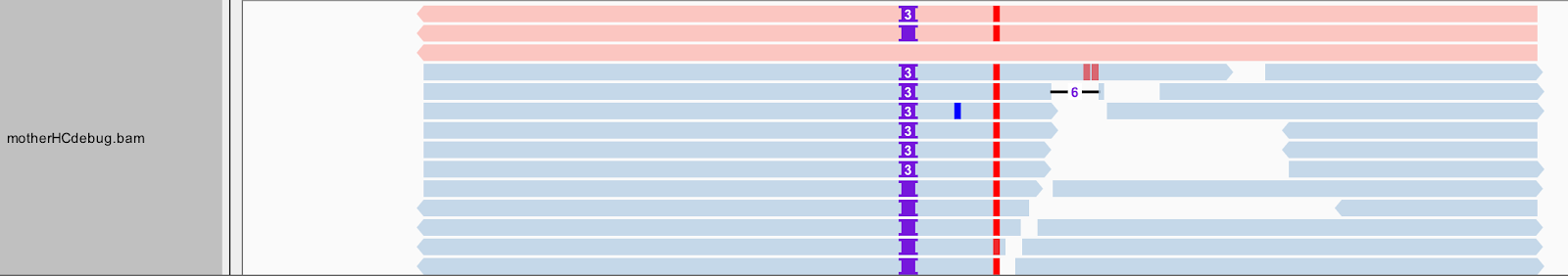
Load the output BAM (sandbox/motherHCdebug.bam) in IGV, and switch to Collapsed view (right-click>Collapsed). You should still be zoomed in on the same coordinates (20:10,002,294-10,002,623), and have the mother.bam track loaded for comparison.
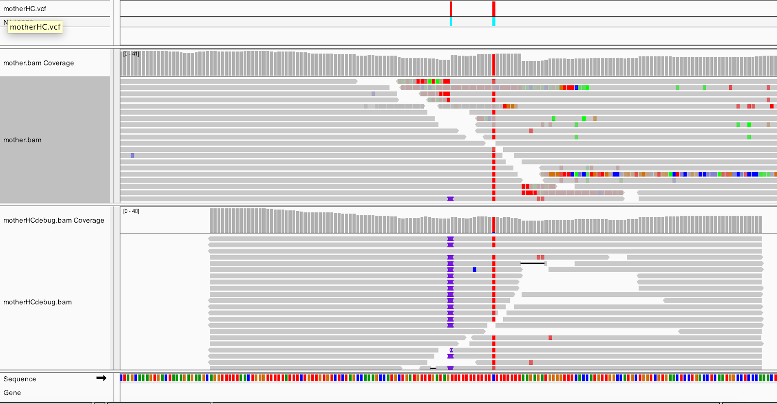
After realignment by HaplotypeCaller (the bottom track), almost all the reads show the insertion, and the messy soft clips from the original bam are gone. HaplotypeCaller will utilize soft-clipped sequences towards realignment. Expand the reads in the output BAM (right-click>Expanded view), and you can see that all the insertions are in phase with the C/T SNP.
This shows that HaplotypeCaller found a different alignment after performing its local graph assembly step. The reassembled region provided HaplotypeCaller with enough support to call the indel, which position-based callers like UnifiedGenotyper would have missed.
➤ Focus on the insertion locus. How many different types of insertions do you see? Which one did HaplotypeCaller call in the VCF? What do you think of this choice?
There is more to a BAM than meets the eye--or at least, what you can see in this view of IGV. Right-click on the motherHCdebug.bam track to bring up the view options menu. Select Color alignments by, and choose read group. Your gray reads should now be colored similar to the screenshot below.
Some of the first reads, shown in red at the top of the pile, are not real reads. These represent artificial haplotypes that were constructed by HaplotypeCaller, and are tagged with a special read group identifier, RG:Z:ArtificialHaplotypeRG to differentiate them from actual reassembled reads. You can click on an artificial read to see this tag under Read Group.
| . | . |
|---|---|
| ➤ How is each of the three artificial haplotypes different from the others? Let's separate these artificial reads to the top of the track. Select Group alignments by, and choose read group. | 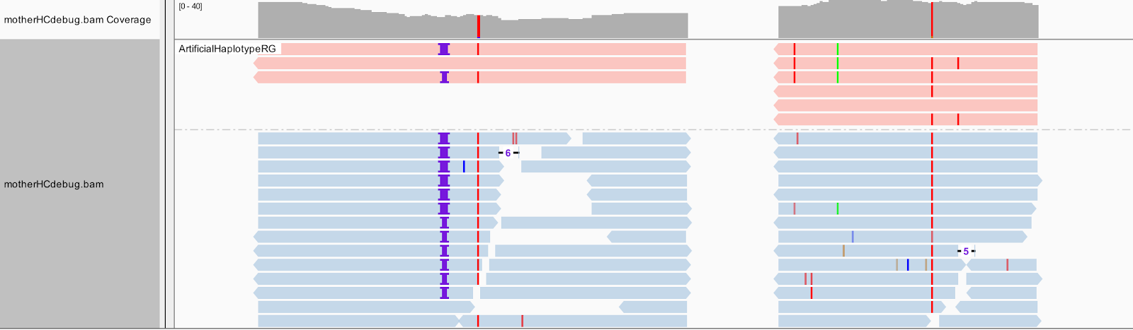 |
Now we will color the reads differently. Select Color alignments by, choose tag, and type in HC. HaplotypeCaller labels reassembled reads that have unequivocal support for a haplotype (based on likelihood calculations) with an HC tag value that matches the HC tag value of the corresponding haplotype.
➤ Again, what do you think of HaplotypeCaller's choice to call the three-base insertion instead of the two-base insertion?
Zoom out to see the three active regions within the scope of the interval we provided. We can see that HaplotypeCaller considered twelve, three, and six putative haplotypes, respectively, for the regions.
GVCF workflow
Run HaplotypeCaller on a single bam file in GVCF mode
It is possible to genotype a multi-sample cohort simultaneously with HaplotypeCaller. However, this scales poorly. For a scalable analysis, GATK offers the GVCF workflow, which separates BAM-level variant calling from genotyping. In the GVCF workflow, HaplotypeCaller is run with the -ERC GVCF option on each individual BAM file and produces a GVCF, which adheres to VCF format specifications while giving information about the data at every genomic position. GenotypeGVCFs then genotypes the samples in a cohort via the given GVCFs.
Run HaplotypeCaller in GVCF mode on the mother’s bam. This will produce a GVCF file that contains likelihoods for each possible genotype for the variant alleles, including a symbolic <NON_REF> allele. You'll see what this looks like soon.
! gatk HaplotypeCaller \
    -R gs://gatk-tutorials/workshop_1903/2-germline/ref/ref.fasta \
    -I gs://gatk-tutorials/workshop_1903/2-germline/bams/mother.bam \
    -O /home/jupyter-user/2-germline-vd/sandbox/mother.g.vcf \
    -ERC GVCF \
    -L 20:10,000,000-10,200,000
# copy files from your notebook sandbox to your workspace bucket sandbox
! gsutil cp -a public-read /home/jupyter-user/2-germline-vd/sandbox/* gs://$BUCKET/sandbox
! echo gs://$BUCKET/sandbox/mother.g.vcf
In the interest of time, we have supplied the other sample GVCFs in the bundle, but normally you would run them individually in the same way as the first.
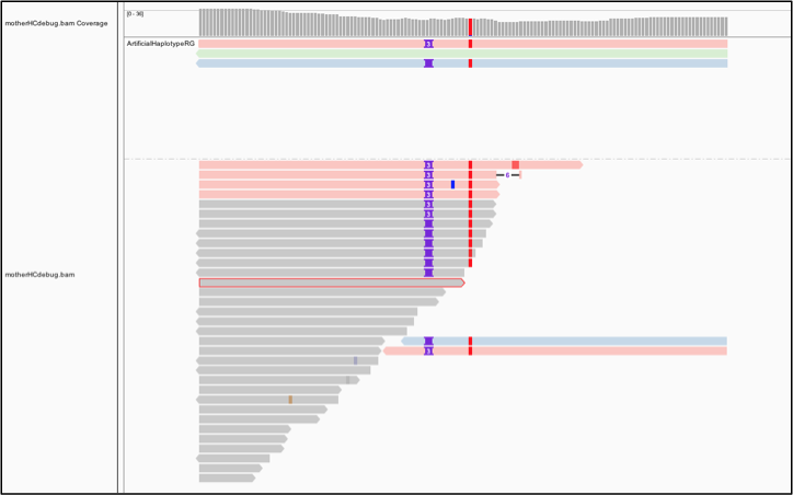
Let's take a look at a GVCF in IGV. Start a new session to clear your IGV screen (File>New Session), then load the GVCF for each family member (gvcfs/mother.g.vcf, gvcfs/father.g.vcf, gvcfs/son.g.vcf). Zoom in on 20:10,002,371-10,002,546. You should see this:
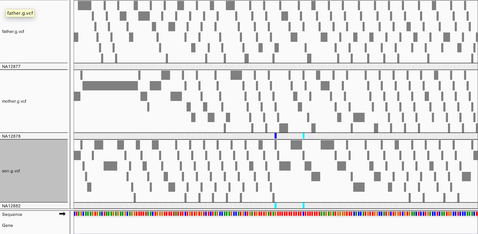
Notice anything different from the VCF? Along with the colorful variant sites, you see many gray blocks in the GVCF representing reference confidence intervals. The gray blocks represent the blocks where the sample appears to be homozygous reference or invariant. The likelihoods are evaluated against an abstract non-reference allele and so these are referred to somewhat counterintuitively as NON_REF blocks of the GVCF. Each belongs to different contiguous quality GVCFBlock blocks.
If we peek into the GVCF file, we actually see in the ALT column a symbolic <NON_REF> allele, which represents non-called but possible non-reference alleles. Using the likelihoods against the <NON_REF> allele we assign likelihoods to alleles that weren’t seen in the current sample during joint genotyping. Additionally, for NON_REF blocks, the INFO field gives the end position of the homozygous-reference block. The FORMAT field gives Phred-scaled likelihoods (PL) for each potential genotype given the alleles including the NON_REF allele.
Later, the genotyping step will retain only sites that are confidently variant against the reference.
Consolidate GVCFs using GenomicsDBImport
For the next step, we need to consolidate the GVCFs into a GenomicsDB datastore. That might sound complicated but it's actually very straightforward.
! gatk GenomicsDBImport \
    -V gs://gatk-tutorials/workshop_1903/2-germline/gvcfs/mother.g.vcf.gz \
    -V gs://gatk-tutorials/workshop_1903/2-germline/gvcfs/father.g.vcf.gz \
    -V gs://gatk-tutorials/workshop_1903/2-germline/gvcfs/son.g.vcf.gz \
    --genomicsdb-workspace-path /home/jupyter-user/2-germline-vd/sandbox/trio \
    --intervals 20:10,000,000-10,200,000
Note: older versions of GenomicsDBImport accept only one interval at a time. Each interval can be at most a contig. To run on a full genome, we would need to define a set of intervals, and execute this command on each interval by itself. See this WDL script for an example pipelining solution. In GATK v4.0.6.0+, GenomicsDB can import multiple intervals per command.
For those who cannot use GenomicDBImport, the alternative is to consolidate GVCFs with CombineGVCFs. Keep in mind though that the GenomicsDB intermediate allows you to scale analyses to large cohort sizes efficiently. Because it's not trivial to examine the data within the database, we will extract the trio's combined data from the GenomicsDB database using SelectVariants.
# Create a soft link to sandbox
! rm -r sandbox
! ln -s /home/jupyter-user/2-germline-vd/sandbox/ sandbox
! gatk SelectVariants \
    -R /home/jupyter-user/2-germline-vd/ref/ref.fasta \
    -V gendb://sandbox/trio \
    -O /home/jupyter-user/2-germline-vd/sandbox/trio_selectvariants.g.vcf
➤ Take a look inside the combined GVCF. How many samples are represented? What is going on with the genotype field (GT)? What does this genotype notation mean?
# copy files from your notebook sandbox to your workspace bucket sandbox
! gsutil cp -a public-read /home/jupyter-user/2-germline-vd/sandbox/* gs://$BUCKET/sandbox
! echo gs://$BUCKET/sandbox/trio_selectvariants.g.vcf
Run joint genotyping on the trio to generate the VCF
The last step is to joint genotype variant sites for the samples using GenotypeGVCFs.
! gatk GenotypeGVCFs \
    -R /home/jupyter-user/2-germline-vd/ref/ref.fasta \
    -V gendb://sandbox/trio \
    -O /home/jupyter-user/2-germline-vd/sandbox/trioGGVCF.vcf \
    -L 20:10,000,000-10,200,000
# copy files from your notebook sandbox to your workspace bucket sandbox
! gsutil cp -a public-read /home/jupyter-user/2-germline-vd/sandbox/* gs://$BUCKET/sandbox
The calls made by GenotypeGVCFs and HaplotypeCaller run in multisample mode should mostly be equivalent, especially as cohort sizes increase. However, there can be some marginal differences in borderline calls, i.e. low-quality variant sites, in particular for small cohorts with low coverage. For such cases, joint genotyping directly with HaplotypeCaller and/or using the new quality score model with GenotypeGVCFs (turned on with -new-qual) may be preferable.
➤ What would the command to run HaplotypeCaller jointly on the three samples look like? How about the command that also produces a reassembled BAM and uses the new quality score model?
gatk HaplotypeCaller \
    -R ref/ref.fasta \
    -I bams/mother.bam \
    -I bams/father.bam \
    -I bams/son.bam \
    -O sandbox/trio_hcjoint_nq.vcf \
    -L 20:10,000,000-10,200,000 \
    -new-qual \
    -bamout sandbox/trio_hcjoint_nq.bam
In the interest of time, we do not run the above command. Note the BAMOUT will contain reassembled reads for all the input samples.
Let's circle back to the locus we examined at the start. Load sandbox/trioGGVCF.vcf into IGV and navigate to 20:10,002,376-10,002,550.

! echo gs://$BUCKET/sandbox/trioGGVCF.vcf
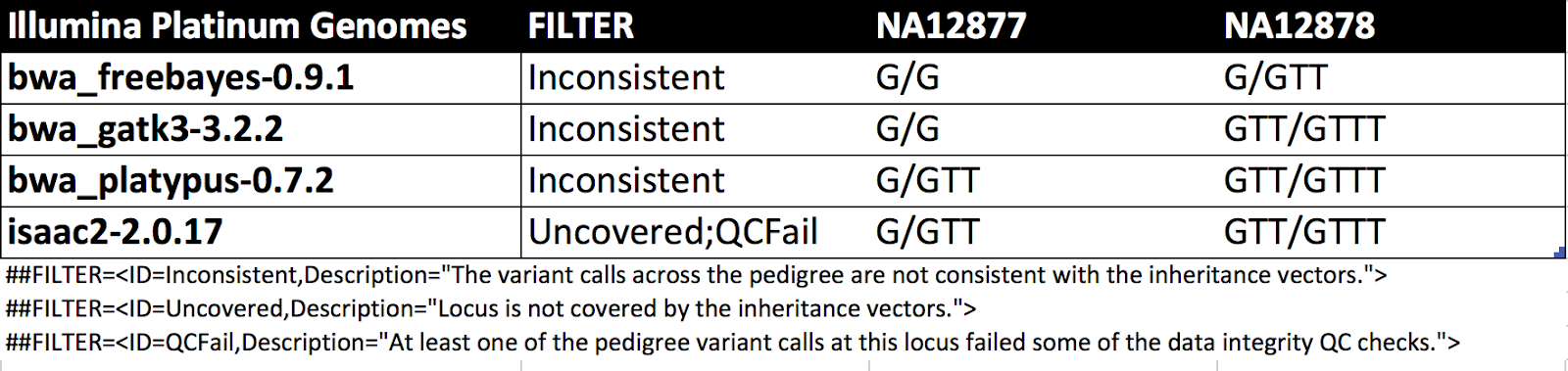
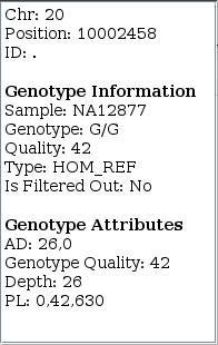
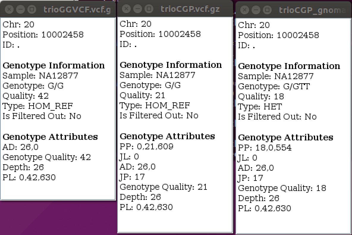
➤ Focus on NA12877's (father) genotype call at 20:10002458. Knowing the familial relationship for the three samples and the child's homozygous-variant genotype, what do you think about the father's HOM_REF call?
Results from GATK v4.0.1.0 also show HOM_REF as well but give PLs (phred-scaled likelihoods) of 0,0,460. Changes in v4.0.9.0 improve hom-ref GQs near indels in GVCFs. The table shows this is an ambiguous site for other callers as well.
| . | . |
|---|---|
 |
 |
GENOTYPE REFINEMENT
Refine the genotype calls with CalculateGenotypePosteriors
We can systematically refine our calls for the trio using CalculateGenotypePosteriors. For starters, we can use pedigree information, which the tutorial provides in the trio.ped file. Second, we can use population priors. For priors we use a population allele frequencies resource derived from gnomAD.
! gatk CalculateGenotypePosteriors \
    -V /home/jupyter-user/2-germline-vd/sandbox/trioGGVCF.vcf \
    -ped /home/jupyter-user/2-germline-vd/trio.ped \
    --skip-population-priors \
    -O /home/jupyter-user/2-germline-vd/sandbox/trioCGP.vcf
! gatk CalculateGenotypePosteriors \
    -V /home/jupyter-user/2-germline-vd/sandbox/trioGGVCF.vcf \
    -ped /home/jupyter-user/2-germline-vd/trio.ped \
    --supporting-callsets /home/jupyter-user/2-germline-vd/resources/af-only-gnomad.chr20subset.b37.vcf.gz \
    -O /home/jupyter-user/2-germline-vd/sandbox/trioCGP_gnomad.vcf
# copy files from your notebook sandbox to your workspace bucket sandbox
! gsutil cp -a public-read /home/jupyter-user/2-germline-vd/sandbox/* gs://$BUCKET/sandbox
! echo gs://$BUCKET/sandbox/trioCGP.vcf
! echo gs://$BUCKET/sandbox/trioCGP_gnomad.vcf
Add both sandbox/trioCGP.vcf and sandbox/trioCGP_gnomad.vcf to the IGV session.
| . | . |
|---|---|
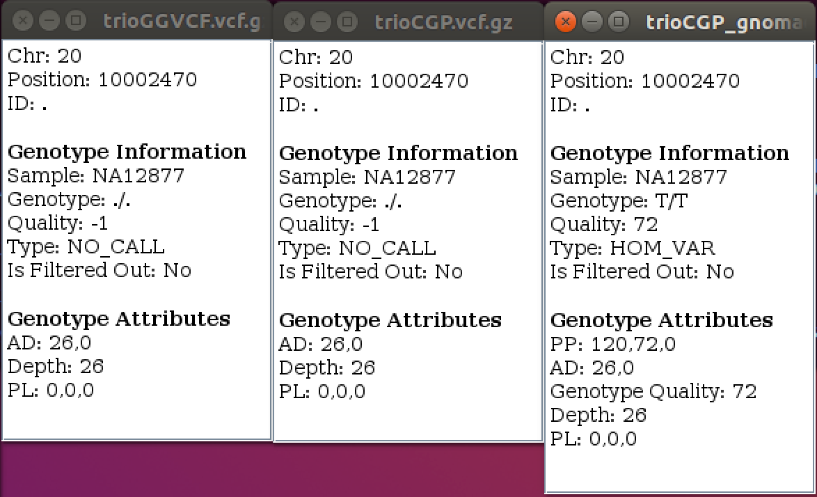
| ➤ What has changed? What has not changed? | 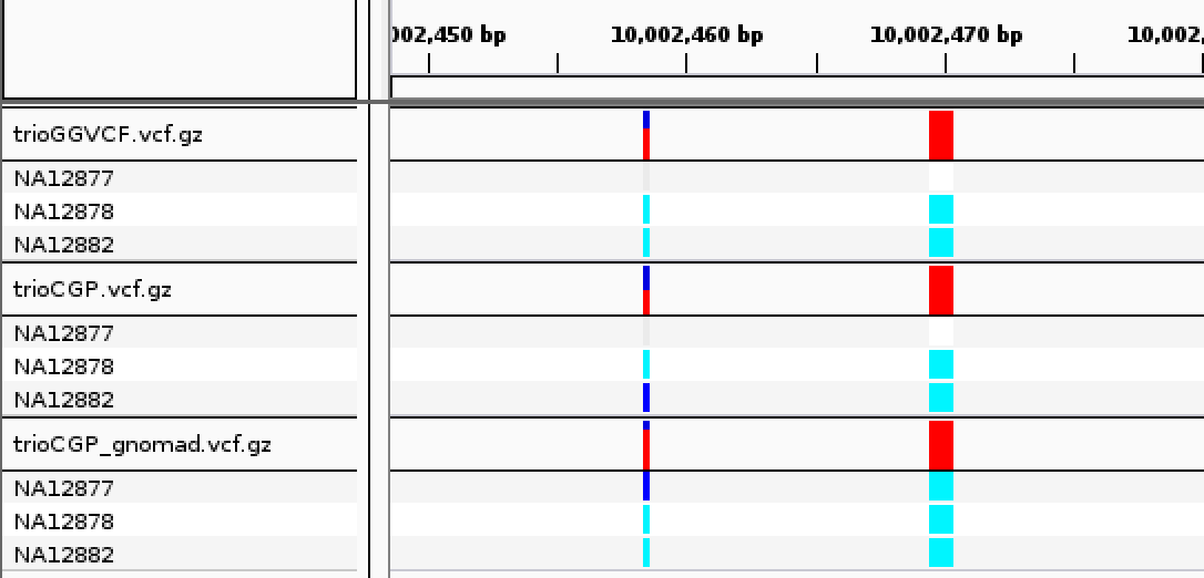 |
CalculateGenotypePosteriors adds three new FORMAT annotations–-PP, JL and JP.
- Phred-scaled Posterior Probability (PP) basically refines the PL values. It incorporates the prior expectations for the given pedigree and/or population allele frequencies.
- Joint Trio Likelihood (JL) is the Phred-scaled joint likelihood of the posterior genotypes for the trio being incorrect.
- Joint Trio Posterior (JP) is the Phred-scaled posterior probability of the posterior genotypes for the three samples being incorrect.
| . | . |
|---|---|
 |
 |
You can learn more about the Genotype Refinement workflow in Article#11074 at https://software.broadinstitute.org/gatk/documentation/article?id=11074.
Compare changes with CollectVariantCallingMetrics
There are a few different GATK/Picard tools to compare site-level and genotype-level concordance that the Callset Evaluation presentation goes over. Here we perform a quick sanity-check on the refinements by comparing the number of GQ0 variants. The commands for the original callset and for that refined with the pedigree are below.
! gatk CollectVariantCallingMetrics \
    -I /home/jupyter-user/2-germline-vd/sandbox/trioGGVCF.vcf \
    --DBSNP /home/jupyter-user/2-germline-vd/resources/dbsnp.vcf \
    -O /home/jupyter-user/2-germline-vd/sandbox/trioGGVCF_metrics
! cat /home/jupyter-user/2-germline-vd/sandbox/trioGGVCF_metrics.variant_calling_summary_metrics
! gatk CollectVariantCallingMetrics \
    -I /home/jupyter-user/2-germline-vd/sandbox/trioCGP.vcf \
    --DBSNP /home/jupyter-user/2-germline-vd/resources/dbsnp.vcf \
    -O /home/jupyter-user/2-germline-vd/sandbox/trioCGP_metrics
! cat /home/jupyter-user/2-germline-vd/sandbox/trioCGP_metrics.variant_calling_summary_metrics
CollectVariantCallingMetrics produces both summary and detail metrics. The summary metrics provide cohort-level variant metrics, while the detail metrics segment the variant metrics for each sample in the callset. The detail metrics give the same metrics as the summary metrics plus the following five additional fields: sample alias, het to homvar ratio, percent GQ0 variants, total GQ0 variants, and total het depth. Metrics are explained at https://broadinstitute.github.io/picard/picard-metric-definitions.html.