Neural Network From Scratch¶

Modules - Modern¶

By Sondre Duna Lundemo, Jenny Lunde, Niels Henrik Aase, Thorvald M. Ballestad, Jon Andreas Støvneng and Brynjulf Owren.

Last edited: March 1st, 2021

---

This notebook will give an introduction to how a fully connected neural network is built, and how the different components work. Throughout the notebook, there will be code snippets for each component in the network, to easier see the connection between the equations and the implementations. Towards the end, all the components will be assembled into classes to make the code more functional and tidy. The problem is based on an excersice in the course TMA4320 - Introduction to Scientific Computation at NTNU.

Remark:¶

If you are unfamiliar with object-oriented programming, don't panic! The way in which classes are used in this notebook will be readily understood by someone with a bit of programming background; you can think of it being a practical way of collecting certain variables together with the functions you use to manipulate them. If you want to learn more you can for instance read more here.

Problem Outline¶

The use of neural networks has had major impact on problems related to artificial intelligence. The general nature of the method makes it perform outstandingly well in a wide variety of tasks, ranging from useful applications such as image recognition and self-driving cars, to less useful applications in for example video games (where the usefulness of video games may be debated!). Another important example where neural networks may be used is to solve classification problems. These kinds of problems also arise in the physical sciences, thus the use of neural networks can in some cases also furnish insight in these fields, insight that is inaccessible if one limits oneself to the conventional methods used in numerical analysis. In a future notebook we will explore such a problem using the vast machinery provided in various Python packages for machine learning. In the present case however, we will implement the algorithms from scratch in order to provide insight into the mechanics of a neural network.

Although the problem does not have to be classification of images, to make the workings of the network less abstract, we will frequently refer to the input of the network as being an image. What we picture, is that each pixel of the image has a scalar value associated to it, say representing a grayscale value. To avoid using matrices as representation of the input, we stack the rows of the image on top of each other to create an input vector, whose dimensions necessarily will be the product of the number of pixels in each direction of the image. In the case of binary classification, the label associated to each image is either $0$ or $1$, and it represents some kind of category. If for example the problem was to be able to say whether an image showed a wolf or a husky, we could translate it to $0$ representing the wolf category and $1$ the husky category.

What Is an Artificial Neural Network?¶

An artificial neural network (ANN) is a set of functions that are put together to mimic a biological neural network [1]. Just as a biological neural network, an ANN consists of many neurons connected together to form a complex network. In an ANN, these neurons are structured in layers. The first is called the input layer, the last layer is called the output layer and between them there is a number of hidden layers$^1$. The number of hidden layers, also known as the depth of the network, will vary depending on the complexity of the problem one want to solve with the network. Each layer holds neurons, and the number of neurons vary from network to network, and it can also vary from layer to layer in a given network.

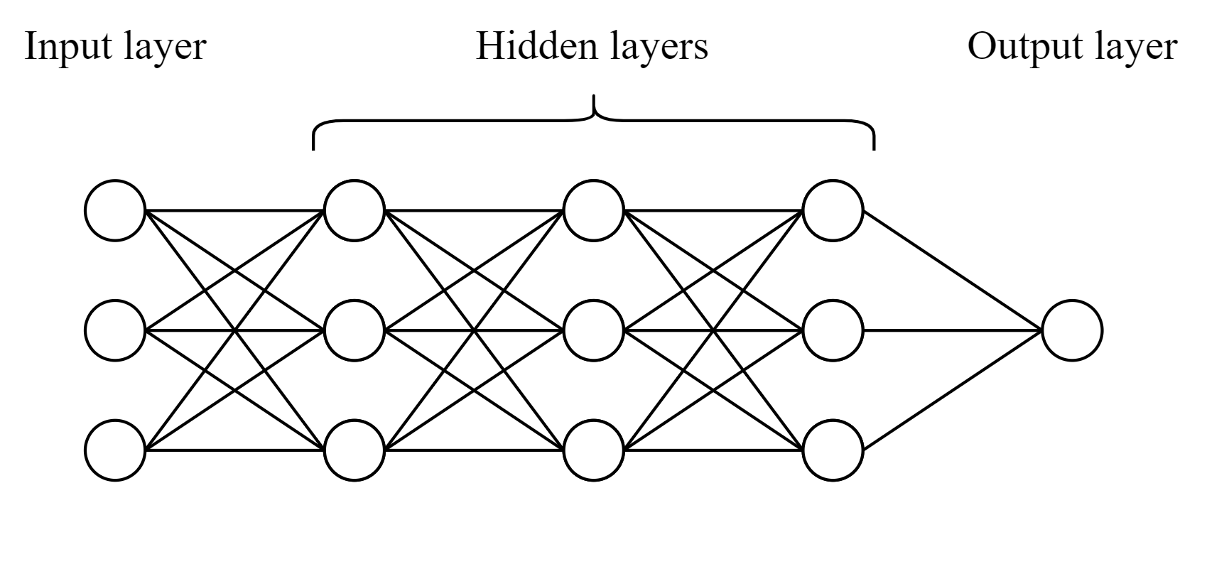This figure is a visualization of the network made in this notebook. The network is fully connected, and the number of neurons is the same for all layers except the output layer. 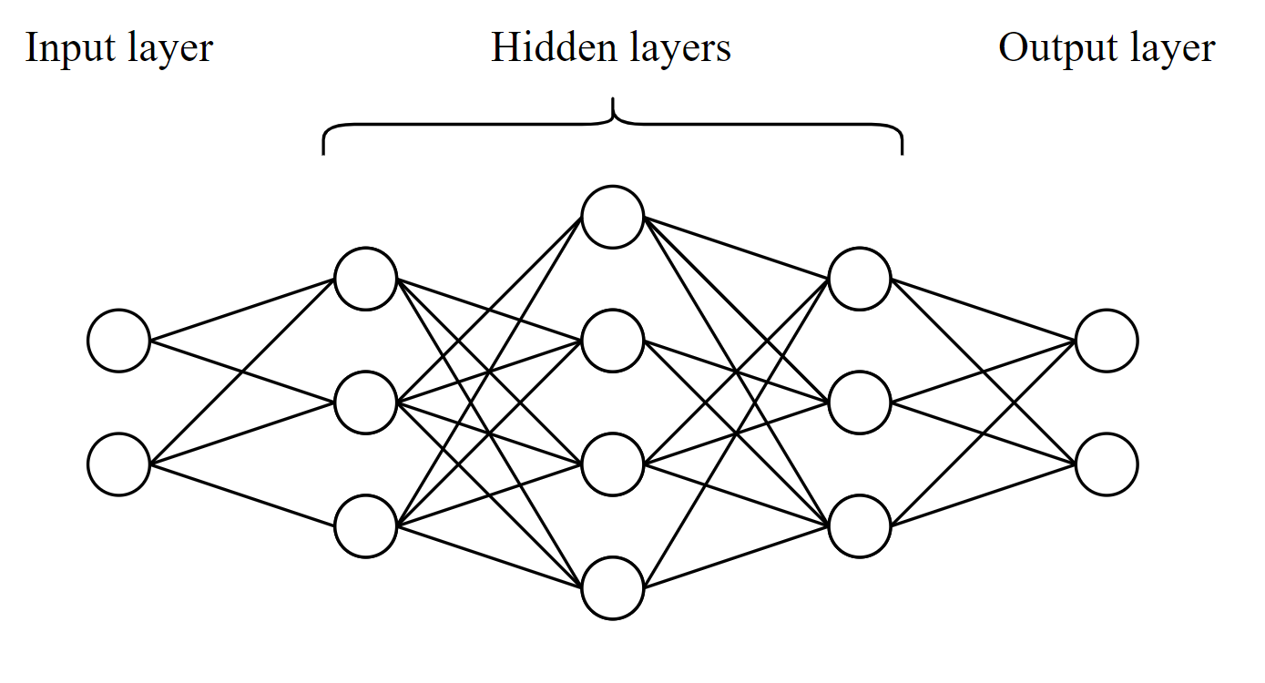This figrue shows a more general neural network. The network is not fully connected, and the number of neurons vary form layer to layer.

We will in this notebook consider an ANN in which the number of neurons in each layer is constant. More specifically, the network we will use is called ResNet, and was first mentioned in this report by Kaiming He, Xiangyu Zhang, Shaoqing Ren and Jian Sun. For simplicity, the number of neurons will be equal to the dimension of the input. We will also restrict our focus to fully connected neural networks, that is, any neuron of the network is connected to all the neurons in the next layer. These simplifications are only made to make the overall structure simpler to implement and understand, but it is important to emphasise that choosing more complicated structures may enhance performance in real applications. For such purposes, using well documented and robust Python packages such as PyTorch or TensorFlow is undoubtedly easier and better than trying to implement the algorithms yourself.

Although the fully connected network is much simpler to implement, it is more computationally expensive than a network that is not fully connected. Another advantage of choosing a more complicated structure is that it allows for treating subsets of the data differently. In that way one can in a sense lead the network into the right path. Furthermore, more complicated structures allow for more complicated and non-linear connections between the neurons.

Overiview of Variables¶

Throughout this notebook, a lot of variables will be introduced. Here is an overview of all of them. The variable names used in the code will be in $\texttt{teletypefont}$.

$$ \begin{equation*} \begin{aligned} K = & \texttt{ num_layers} && \text{ Number of layers.} \\ I = & \texttt{ num_images} && \text{ Number of images.} \\ d = & \texttt{ dimension} && \text{ Dimension of input data.} \\ Y = & \texttt{ Y} && \text{ All output values, } y \text{, in a matrix of size [num layes + 1, num neurons]. } Y[0] \text{ is the input to the network.} \\ W = & \texttt{ weight} &&\text{ All weights, } w \text{, in a matrix of size [num layers, num neurons, num neurons].} \\ B = & \texttt{ bias_vec} &&\text{ All biases, } b \text{, in a matix for size [num layers, num neurons].} \\ \mu = & \texttt{ mu} &&\text{ Variable corresponding to a bias in the output layer.}\\ \omega = & \texttt{ omega} &&\text{ Variable corresponding to a weight in the output layer.}\\ h = & \texttt{ steplength} &&\text{ Steplength.} \\ Z_i = & \texttt{ Z} &&\text{ Output from last layer, the 'guess' of the network.} \\ c_i = & \texttt{ c} &&\text{ The correct value for an output.}\\ \mathcal{J} = & \texttt{ cost_function} &&\text{ The error/cost of the network.}\\ U = & \texttt{ U} &&\text{ Collection of all variables} W \text{, } b\text{, } \omega \text{ and } \mu \text{.}\\ \sigma = & \texttt{ sigma} &&\text{ Sigmoid function, but used generally as activation function.} \\ \eta = & \texttt{ eta} &&\text{ Projection function for output layer.} \\ \sigma ' = & \texttt{ sigma_derivative} &&\text{ The derivative of the activation function.} \\ \eta ' = & \texttt{ eta_derivative} &&\text{ The derivative of the projection function.} \\ \end{aligned} \end{equation*} $$

Since what we end up with is essentially a collection of many variables that we want to manipulate in different ways, and in specific orders, it is convenient to gather these in a class. In this notebook, we have made three classes which we will call $\texttt{Network}$, $\texttt{Param}$ and $\texttt{Gradient_descent}$, and the content of the classes will be explained along the way.

How Does a Layer in the Network Work?¶

In the following, $k$ will denote the index of an arbitrary layer, $n$ an arbitrary neuron index and $i$ an arbitrary index for input vectors to the network. $K$ denotes the total number of layers and $N$ is the total number of nodes in each layer.

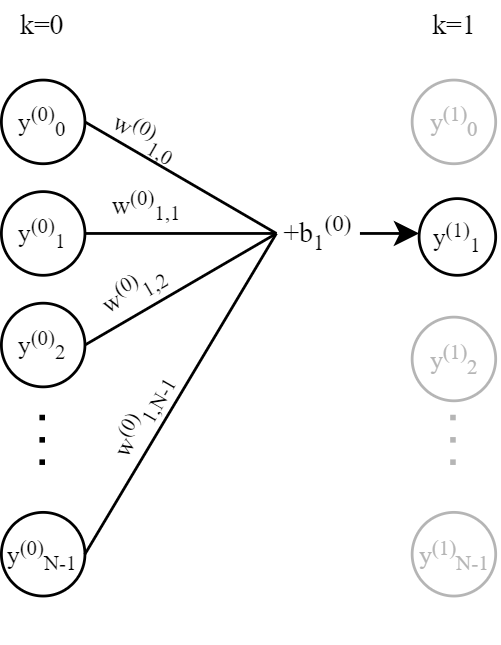This figure shows how the previous layer is the input to a node in the current layer. The variable $k$ is the number of the current layer, and corresponds to the superscript of $y$. The subscript of $y$ is $n$, which tells us what neuron in the layer $y_n$ corresponds to.

Each layer takes in input form the previous layer, except the first layer which takes in the input to the network. In a fully connected layer, each neuron takes the output from every neuron in the previous layer as input. In a neuron, every input is multiplied by an individual weight and then they are all summed up. A bias is added to the sum, and then the results is passed through an activation function before it is sent as output to the next layer together with the output form every other neuron in the same layer. Why is a neuron built up like this? As mentioned in the beginning, an ANN is made to mimic a biological neural network, and in a biological neural network different stimuli 'light up' different neurons, and the signal is passed on to specific neurons. In an ANN the output value from a neuron can be interpreted as if the neuron has been 'lit up' or not. Values close to 1 means 'lit up' while values close to 0 represent an inactive neuron$^2$. By denoting the inputs to the first layer by $y^{(0)}_n$, the weights to each input to the a neuron in the first layer $w_{0,n}^{(0)}$, the bias $b_0^{(0)}$ and the activation function $f$, the output of neuron $1$ will be

$$ y^{(1)}_0 = y^{(0)}_0 + h f\big( w_{0,0}^{(0)} y^{(0)}_0 + w_{0,1}^{(0)} y^{(0)}_1 + w_{0,2}^{(0)} y^{(0)}_2 + \dots + w_{0,N-1}^{(0)} y^{(0)}_{N-1} + b_0^{(0)} \big) \text{.} $$

$h$ is known as the steplength, and is a number between 0 and 1. It is the combination of the output value from each neuron in the previous layer and their corresponding weights that affect the sum in the present neuron. The bias can push the value up or down to effectively make a threshold for activation. After having transformed the input through the hidden layers, it is passed through an activation function which projects the output on a scalar between 0 and 1 in the case of binary classification. One example of an activation function is the sigmoid function:

$$ \sigma(x) = \frac{1}{1 + e^{-x}}. $$

To simplify notation and calculations, matrices and vectors are used to compactly gather the weights and biases. Let the inputs to the first layer be the vector $y^{(0)}$, $W^{(0)}$ be a matrix with the weights in the first layer and $b^{(0)}$ be the biases in the first layer. $W$ consist of vectors with the weights from each neuron in the layer. The output from the first layer is then in matrix notation

$$ \begin{equation*} \begin{aligned} \begin{bmatrix} y^{(1)}_0\\ y^{(1)}_1\\ \vdots \\ y^{(1)}_{N-1}\\ \end{bmatrix} = \begin{bmatrix} y^{(0)}_0\\ y^{(0)}_1\\ \vdots \\ y^{(0)}_{N-1}\\ \end{bmatrix} + h \sigma \left( \begin{bmatrix} w^{(0)}_{0,0} & w^{(0)}_{0,1} & \dots & w^{(0)}_{0,N-1} \\ w^{(0)}_{1,0} & w^{(0)}_{1,1} & \dots & w^{(0)}_{1,N-1} \\ &\vdots \\ w^{(0)}_{N-1,0} & w^{(0)}_{N-1,1} & \dots & w^{(0)}_{N-1,N-1} \\ \end{bmatrix} \begin{bmatrix} y^{(0)}_0\\ y^{(0)}_1\\ \vdots \\ y^{(0)}_{N-1}\\ \end{bmatrix} + \begin{bmatrix} b^{(0)}_0\\ b^{(0)}_1\\ \vdots \\ b^{(0)}_{N-1}\\ \end{bmatrix} \right) \text{,} \end{aligned} \end{equation*} $$

or written more compactly

$$ y^{(1)} = y^{(0)} + h \sigma \left(W^{(0)}y^{(0)} + b^{(0)}\right) \text{,} $$

where the sigmoid function$^3$, $\sigma$, is applied elementwise. In a fully connect neural network every neuron in one layer is connected to every neuron in the next layer, and the matrix equation above gives the output of each hidden layer in the network. It is convenient for computational purposes to send every input-vector through the transformation simultaneously. In our notation, this amounts to

\begin{equation} \mathbf{Y}_{k} = \mathbf{Y}_{k-1} + h \sigma \left( W_{k-1} \mathbf{Y}_{k-1} + b_{k-1}\right). \end{equation}

Activation Functions¶

Activation functions are what differentiate a neural network from linear regression. Without processing the output from each layer through a non-linear activation function, it would always be possible to make a single layer that is equal to the sum of any other set of layer of the same size, and the depth of the network would be insignificant. With the use of activation functions, it is possible for the network to make non-linear connections between the input and the output. Another aspect of the activation function is that it becomes more clear whether the neuron is active or inactive. One could think that the best way to show this would be a binary activation function that outputs 1 if it is active and 0 else, but then the gradient of the function will be ill-defined. It will become clear that this is very unfortunate when we discuss training of the network, where the gradient of the activation function plays a crucial role. There are many choices for activation functions, some of the most well known are sigmoid function, hyperbolic tangent and the ReLU function.

Sigmoid¶

The sigmoid function is a well known activation function, and it outputs values between 0 and 1. It is a continuous function and makes gradient calculations simple. One downside with this function is what is called 'vanishing gradients'. That is, when the absolute value of the input takes a large value, the gradient of the sigmoid function gets very small. As we will see later, the gradient of the activation function is an important part of the learning of the network, and vanishing gradients will make the network learn very slowly [2]. The function can also be used in the output layer.

Hyberbolic Tangent¶

The shape of the hyperbolic tangent function is similar to the sigmoid function, but it takes values between $-1$ and $1$. According to [3], centering the values around 0 will make the network learn easier, and it often gives better results than the sigmoid function.