Relaxation Methods
Modules – Partial Differential Equations
Last edited: February 7th 2018 ___Relaxation methods involves solving the system of equations that arises from a finite difference approximation iteratively until a solution is found [1]. We will introduce the Jacobi method, the Gauss-Seidel method and succesive overrelaxation (SOR). The methods can be used to solve an elliptic equation
$$\mathcal L \psi = \rho,$$where $\mathcal L$ is an elliptical operator and $\rho$ is a source term.
The methods are simple to understand through a concrete example. We will be solving the two-dimensional Poisson equation,
\begin{equation} \nabla^2 \psi(x, t) = \frac{\partial^2 \psi(x, y)}{\partial x^2} + \frac{\partial^2 \psi(x, y)}{\partial y^2} = \rho(x, y), \label{eq:poisson} \end{equation}for a square domain $\Omega = (0,L)\times (0, L)$, $L\in \mathbb R_+$. Without loss of generality we let $L=1$.
The Poisson Equation in Physics
The Poisson and Laplace $(\rho = 0)$ equations are widely used in physics. In electrostatics, the electric potential is described by $\nabla^2 V\left(\mathbf r\right) = -\rho \left(\mathbf r\right)/\epsilon_0,$ where $V$ is the electric potential and $\epsilon$ is the electric permittivity (this is the differential form of Gauss' law for the electric potential. See e.g. [2]). The steady state of the diffusion equation becomes $u_t = \nabla^2 u - \rho = 0$. For a steady incompressible flow in two dimensions, the stream function satisfies $\nabla^2 \psi = -\zeta$, where $\zeta=\nabla\times \mathbf V$ is the vorticity and the velocity field is given by $\mathbf V = (u, v) = (\psi_y, -\psi_x)$ (See e.g. [3]).
The solution is unique when the boundary conditions for the entire system is well defined. This is discussed in more detail in the appendix below.
Jacobi Method
Consider the equation
\begin{equation} \frac{\partial \psi(x, y, t)}{\partial t}=\frac{\partial^2 \psi(x, y, t)}{\partial x^2} + \frac{\partial^2 \psi(x, y, t)}{\partial y^2} - \rho(x, y), \label{eq:diffusion} \end{equation}whose steady state is the Poisson equation \eqref{eq:poisson}. Let $x$, $y$ be discretized to some grid,
$$x_i = x_0 + i\Delta x, \: (\:i=0, 1, ...,N)$$$$y_i = y_0 + j\Delta y, \: (\:j=0, 1, ..., N)$$and let, $$t_n = n\,\delta t, \: (\:n = 0, 1, ..., n).$$
Since we are considering the square domain $\Omega$, we have $x_0 = y_0 = 0$ and $x_n = y_m = 1$. To simplify the notation we introduce $u(x_i, y_j, t_n)\equiv u_{i, j}^n$ and $\rho(x_i, y_j) \equiv \rho_{i, j}$.
If we use central differencing in space and and foreward differencing in time (FTCS) on equation \eqref{eq:diffusion}, we get
$$\frac{\psi^{n+1}_{i, j} - \psi^n_{i, j}}{\Delta t} = \frac{\psi^n_{i+1, j}-2\psi^n_{i, j}+\psi^n_{i-1, j}}{(\Delta x)^2} + \frac{\psi^n_{i, j+1}-2\psi^n_{i, j}+\psi^n_{i, j-1}}{(\Delta y)^2} - \rho_{i, j}.$$For convinience we let $\Delta \equiv \Delta x=\Delta y$. We then obtain
\begin{equation} \psi^{n+1}_{i, j} = \psi^n_{i, j} + \frac{\Delta t}{\Delta^2} \left(\psi_{i+1, j}^n + \psi_{i-1, j}^n + \psi_{i, j+1}^n + \psi_{i, j-1}^n - 4\psi_{i, j}^n\right) - \Delta t \,\rho_{i, j}. \label{eq:poisson_differenced} \end{equation}It can be shown that the FTCS differencing for the Poisson equation in two dimensions is stable only if $\Delta t/\Delta^2 \leq 1/4$ (see Appendix). If we set $\Delta t/\Delta^2 = 1/4$ we get
\begin{equation} \psi^{n+1}_{i, j} = \frac{1}{4} \left(\psi_{i+1, j}^n + \psi_{i-1, j}^n + \psi_{i, j+1}^n + \psi_{i, j-1}^n\right) - \frac{\Delta ^2}{4} \,\rho_{i, j}. \label{eq:jacobi_method} \end{equation}The algorithm thus consists of choosing the value at $(x_i,y_j)$ as the average of the neighboring points plus some source term $\rho$.
We can use any initial guess. The iteration is repeated until a convergence criterion is met. We will be using the total relative change between two iterations as a stopping condition. The final solution is the steady state solution of equation \eqref{eq:diffusion}, which is the Poisson equation \eqref{eq:poisson}.
Example
Consider a square domain without any sources. The Poisson equation reduces to the Laplace equation $(\rho = 0)$ inside the domain. The boundary conditions are indicated in figure 1 below. We choose $L=1$, $a=0$ and $b = 1$ (with the necessary dimensions) without loss of generality.
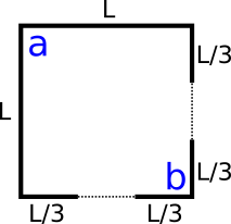 Figure 1: Setup used in the example. The value of $\psi$ along the solid lines are $a$ and $b$ as indicated. $\psi$ vary evenly between $a$ and $b$ along the dotted lines.
This setup can for example model a conductor (the upper left part, $a$) and a conductor with a uniformly distributed charge (the lower right part, $b$). The electric field is in turn given by $\mathbf E = \nabla \psi$. The setup can also model the flow of an incompressible and irrotational fluid through a square cavity with uniformal inflow and outflow. The inflow and outflow being the dottet lines, respectivaly the right and bottom. The velocity field is given by $\mathbf V = (\partial_y \psi, - \partial_x \psi)$. We refer you to our seperate notebooks on stream functions and electromagnetism for more information.
To solve the Laplace equation for this setup we use the Jacobi method. We define the following functions.
import numpy as np

def bc(n=32):
    """ Represents the boundry conditions of psi as in the setupin figure 1
        in a 2D matrix.

    Parameters:
        n :     int. Number of discretisations in the x- and y-
                direction
    Returns:
    int array, size (n, n). The boundry conditions.
    """

    psi = np.zeros((n, n))
    width = int(n/3)

    # Boundary conditions
    psi[0, 2*width:] = 1  # Lower left part of b
    psi[:width, -1] = 1   # upper right part of b
    psi[0, width:2*width] = np.linspace(0, 1, width)  # Inflow
    psi[width:2*width, -1] = np.linspace(1, 0, width) # Outflow
    # The rest are already zero

    return psi

def jacobi(n=32, maxit=1000, tol=1e-10):
    """ This function uses Jacobi's method to solve the Poisson
    equation for the square domain and boundary conditions as
    indicated in the figure.

    Parameters:
        n :     int. Number of discretisations in the x- and y-
                direction
        maxit : int. Maximum number of iterations.
        tol :   float. Tolerance in convergence criterion.
                If the total relative change between two
                iterations are less that 'tol', we say that
                the method has converged.
    Returns:
    float array, size(n, n). The estimated solution.
    """

    psi = bc(n)
    psi_temp = psi.copy()
    itnum = 1             # Iteration counter
    change = tol + 1      # Total relative quadratic change between each iteration

    for itnum in range(maxit):
        # Let each point be the mean of its nearest neighbors
        psi_temp[1:-1, 1:-1] = .25*(psi[2:, 1:-1] + psi[:-2, 1:-1] +
                                    psi[1:-1, 2:] + psi[1:-1, :-2])
        # Update the convergence check for every 50 iteration
        if itnum % 50 == 0:
            if np.sum(np.abs(psi_temp - psi))/np.sum(psi) < tol:
                print("Iterations: ", itnum + 1)
                break
        psi = psi_temp.copy()

    if itnum == maxit - 1:
        print("Maximum number of iterations (%i) reached!"%(maxit))

    return psi
Let's perform one example.
n = 64
tol = 1e-5
psi = jacobi(n, maxit=10000, tol=1e-5)
Iterations: 3551
We then visualize the result for the two physical interpretations mentioned above.
# Needed package
import matplotlib.pyplot as plt
plt.style.use('bmh')
%matplotlib inline

def plot(psi, n):
    # Compute the gradient. v=psi_yy, u=psi_xx
    v, u = np.gradient(psi)

    x = np.linspace(0, 1, n) # x-axis
    vmag = np.sqrt(u**2 + v**2)

    # Create figure
    fig, axarr = plt.subplots(1, 2, figsize=(10, 6), dpi=300)

    # Axes 1: Electric potential and field
    im1 = axarr[0].contourf(x, x, psi, 20)
    axarr[0].streamplot(x, x, -u, -v, color="k")
    axarr[0].set_title("Electric potential and field")
    fig.colorbar(im1, orientation='horizontal', ax=axarr[0],
                  label=r"Electric potential, $V/V_0$")
    axarr[0].set_xlabel("$x/L$")
    axarr[0].set_ylabel("$y/L$")

    # Axes 2: Velocity field and strength
    # Flow of an incompressible and irrotational fluid
    im2 = axarr[1].contourf(x, x, vmag/np.max(vmag), 20)
    axarr[1].streamplot(x, x, v, -u, color="k")
    axarr[1].set_title("Velocity field and strength")
    fig.colorbar(im2, orientation='horizontal', ax=axarr[1],
               label=r"Velocity magnitude, $v/v_0$")
    axarr[1].set_xlabel("$x/L$")
    axarr[1].set_ylabel("$y/L$")
    axarr[1].set_xlim([0, 1])
    axarr[1].set_ylim([0, 1])
plot(psi, n)

General Case
The Jacobi method can used to solve a general matrix equation $A\mathbf x = \mathbf b$ (assuming that the method converges). Let $D$ be the diagonal part of $A$, $L$ be the lower triangular part of $A$ and $U$ be the upper triangular part of $A$. Then, the Jacobi method can be written as
\begin{equation} D\mathbf x^{\,(k+1)} = -(L+U)\mathbf x^{\,(k)} + \mathbf b. \end{equation}In the example above $D$ was simply the unit matrix, and $\mathbf b$ was the source term $\rho$ (with a reindexing, $\rho_{i, j}\to \rho_{i+jN}$).
The Gauss-Seidel Method
The Gauss-Seidel method is similar to the Jacobi method, but the average at each point is computed with the "newest" available data. If the averaging is performed along the $x$-axis ($i$ varying, $j$ fixed), then
\begin{equation} \psi^{n+1}_{i, j} = \frac{1}{4} \left(\psi_{i+1, j}^n + \psi_{i-1, j}^{n+1} + \psi_{i, j+1}^n + \psi_{i, j-1}^{n+1}\right) - \frac{\Delta ^2}{4} \,\rho_{i, j}. \label{eq:gauss-seidel_method} \end{equation}In matrix form, the Gauss-Seidel method is
\begin{equation} (L+D)\mathbf x^{\,(k)} = -U\mathbf x^{\,(k-1)}+ \mathbf b. \label{eq:gauss-seidel_matrix} \end{equation}Successive Overrelaxation (SOR)
The Gauss-Seidel method \eqref{eq:gauss-seidel_matrix} can be rewritten as
$$\mathbf x^{\,(k)} = \mathbf x^{\,(k-1)} - (L + D)^{-1}\mathbf \xi^{\,(r-1)},$$where $\mathbf \xi^{\,(r-1)}=\left[(L+D+U)\mathbf x^{\,(r-1)}-\mathbf b\right]$. $\xi$ is simply a residual vector which we overcorrect by introducing a overrelaxation parameter $\omega$. The SOR method can thus be written as
\begin{equation} \mathbf x^{\,(k)} = \mathbf x^{\,(k-1)} - \omega (L + D)^{-1}\mathbf \xi^{\,(r-1)}. \end{equation}It can be proved that the SOR method is convergent only for $0<\omega < 2$ and only $1<\omega < 2$ can give a faster convergence than the Gauss-Seidel and Jacobi methods [1] (see Appendix for a quick review of the convergence rates). The method is called underrelaxed if $0<\omega < 1$. One disadvantage of this method is that the optimal value for $\omega$ is in general not known analytically. In these cases one can find an approximate value empirically.
Let us create a function that performs the same computations as the example above, to compare the Jacobi method and SOR. Note that we cannot use Numpy-arrays to optimize the computation speed for the SOR and Gauss-Seidel methods. Thus, the number of iterations may be less, but the computational time is much larger than that of the Jacobi method. This "problem" is resolved if we use a compiled language such as fortran, C or C++ (see e.g. our tutorial on F2PY for more information).
We can use the residual as a check for convergence. In order to compare the two methods we have used, we will stop the iterations if the total relative change between two iterations is below a given tolerance as we did before.
def sor(n=32, omega=1, maxit=1000, tol=1e-5):
    """ This function uses successive overrelaxation (SOR) to
    solve the Poisson equation for the square domain and
    boundary conditions as indicated in figure 1.

    Parameters:
        n :     int. Number of discretisations in the x- and y-
                direction
        omega:  float. Overrelaxation parameter (0 < omega < 2)
        maxit : int. Maximum number of iterations.
        tol :   float. Tolerance in convergence criterion.
                If the total relative change between two
                iterations are less that 'tol', we say that
                the method has converged.
    Returns:
    float array, size(n, n). The estimated solution.
    """

    psi = bc(n) # Get initial guess and boundry conditions

    for itnum in range(maxit):
        total_xi = 0
        for i in range(1, n - 1):
            for j in range(1, n - 1):
                xi = psi[i + 1, j] + psi[i - 1, j] + psi[i, j + 1] + psi[i, j - 1] - 4*psi[i, j]
                total_xi += abs(xi)
                psi[i, j] += omega*xi/4
        if .25*total_xi/np.sum(psi) < tol:
            print("Iterations: ", itnum + 1)
            break

    if itnum == maxit - 1:
        print("Maximum number of iterations (%i) reached!"%(maxit))

    return psi
n = 64
w = 1.91 # Approximation of the optimal value after a few tests
psi = sor(n, omega=w, maxit=1000, tol=5e-5)
Iterations: 92
plot(psi, n)

As conclusion, SOR required a lot fewer iterations than the Jacobi method. Note that the stopping criterion in SOR is in fact somewhat stricter than that of the Jacobi method, since the convergence rate is higher.
Chebychev Acceleration
There are a few simple methods to improve the SOR algorithm. A given optimal value for $\omega$ for the asympotic behaviour is not necessarily a good choice for inital value. There is a clever prescription for choosing a value $\omega$ that changes for each iteration. In addition, you may note that the "odd" meshes do only depend on the previous values of the "even" meshes, and vice versa. A SOR with these optimalizations is called Chebychev acceleration [1].
Resources and Further Readings
[1] William H. Press, Saul A. Teukolsky, William T. Vetterling, and Brian P. Flannery. Numerical Recipes 3rd Edition: The Art of Scientific Computing. Cambridge University Press, 3 edition, September 2007.
[2] David J. Griffiths. Introduction to Electrodynamics (3rd Edition). Benjamin Cummings, 1998.
[3] F. Durst. Fluid Mechanics an Introduction to the Theory of Fluid Flows. Springer-Verlag Berlin Heidelberg. 2008. https://doi.org/10.1007/978-3-540-71343-2
Appendix
Uniqueness Theorem for Poisson Equation
Consider the Poisson equation
$$\nabla^2\psi(\mathbf r) = -\rho(\mathbf r)_f,$$for some real potential $\psi$ and source term $\rho$. Suppose that there are two distinct solutions $\psi_1(\mathbf r)$ and $\psi_2(\mathbf r)$. By taking the difference of the Poisson equation for each of the solutions, we obtain
$$0 = \nabla^2\psi_1(\mathbf r) - \nabla^2\psi_2(\mathbf r) = \nabla^2\left[\psi_1(\mathbf r) - \psi_2(\mathbf r)\right].$$Define $\phi(\mathbf r)\equiv \psi_1(\mathbf r) - \psi_2(\mathbf r)$. Notice that
$$\nabla (\phi\nabla\phi)=(\nabla\phi)^2+ \phi\nabla^2\phi=(\nabla\phi)^2.$$We now take the integral over some volume $V$ bounded by a surface $S$ on both sides:
$$\int_V\mathrm{d}^3\mathbf{r}\;(\nabla\phi)^2=\int_V\mathrm{d}^3\mathbf{r}\;\nabla(\phi\nabla\phi).$$The last integral can be rewritten as a surface integral over $S$ by using the divergence theorem. We thus obtain
$$\int_S \phi\nabla\phi\cdot \mathrm d\mathbf a = \int_V\mathrm{d}^3\mathbf{r}\;(\nabla\phi)^2.$$Note that $(\nabla \phi)^2\geq 0$ everywhere, which implies that $\nabla \phi=0$ everywhere if
$$\int_S \phi\nabla\phi\cdot \mathrm d\mathbf a=0.$$In other words, the gradient of the solution is unique when the surface integral vanishes. This is the case when $\phi$ or $\nabla \phi$ is specified at the boundaries. This is called Dirichlet and Neumann boundary conditionds, respectively. The boundary conditions can also be described at $r\to \infty$ if the surface integral vanishes.
The uniqueness theorem for the Laplace equation for electromagnetism is discussed in ref. [2].
Von Neumann Stability Analysis for the FTCS Differencing Scheme of the Poisson Equation
Following is a short application of the Von Neumann Stability Analysis for the FTCS (Forward Time, Centerered Space) finite differencing. In short, it consists of linearlizing the equation and seperating the spacial and time dependent parts and look at the locally error growth. For more information and a deeper insight see e.g. [chap. 20, 1].
Assume that the solutions to the difference equation can be written as
\begin{equation} \psi^n_{j, l}=\xi^n(k, q)e^{ikj\Delta x}e^{iql\Delta y}, \label{eq:fourier} \end{equation}where $i$ is the imaginary unit and $k$ and $q$ are real numbers. The growth factor $G=\xi^{n+1}/\xi^n$ of the scheme is found by substituting the expression above into the difference equation. The method is stable if $|G|\leq 1$ for all real $k$ and unstable if $|G|>1$ some real $k$.
In our case we must insert \eqref{eq:fourier} into \eqref{eq:poisson_differenced} and use $\Delta \equiv\Delta x = \Delta y$. In areas with no source ($\rho = 0$), the result is
$$ \begin{aligned} G &= 1 + 2\frac{\Delta t}{\Delta^2}\left(\cos(k\Delta) + \cos(q\Delta) - 2\right)\\ &=1 - 4\frac{\Delta t}{\Delta^2}\left(\sin^2(k\Delta/2) + \sin^2(q\Delta/2)\right). \end{aligned} $$If we require that $|G|\leq 1$ for all $k$ and $q$ we obtain the stability criterion
\begin{equation} \frac{\Delta t}{\Delta^2}\leq \frac{1}{4}. \end{equation}Convergence Rate
The Jacobi and Gauss-Seidel methods are both slowly converging. It can be shown that the number of iterations $r$ required to reduce the error by a factor $10 ^{-p}$ is estimated by
\begin{align*} r&\approx \frac{1}{2}pN^2\quad\text{(Jabobi)}, \\ r&\approx \frac{1}{4}pN^2\quad\text{(Gauss-Seidel)}, \end{align*}where $N^2$ is the number of mesh points [1]. The SOR method is in general much faster than the Jacobi and Gauss-Seidel methods for an optimal parameter $\omega$, for which it only requires an order of $N$ iterations. It can be shown that the optimal value for $\omega$ at large $N$ can be estimated by
$$\omega_\text{opt}\approx\frac{2}{1+\pi/N},$$and that
\begin{equation*} r\approx \frac{1}{3}pN\quad\text{(SOR)}, \end{equation*}for the setup used in the examples [1].