Tomography
Examples – Biophysics
Last edited: January 20th 2019This notebook is based on an assignment given in the course TMA4320 Introduction to Scientific Computation at NTNU in April 2016 [1]. The assignment was prepared by Pål Erik Goa, Jon Andreas Støvneng, Peder Galteland and Grunde Wesenberg. The code is based on the answers by Gjert Magne Knutsen, Daniel Halvorsen and Jonas Tjemsland. ___
Introduction
Medical imaging is central in modern diagnostics. Fig. 1 below shows a cross section of a head based on so-called computed tomography (CT). In this notebook we get a glimpse off how CT uses X-rays to reconstruct quite sharp images. We will use grayscaled images of size $N\times N$, which is represented by an $N\times N$ matrix. The value of each matrix element will represent the "grayness" of the pixel ($1$ for white and $0$ for black). In the end we will use the tools developed in the notebook Image Filtering Using Fourier Transform to get a sharper image.
 **Figure 1:** *Axial CT scan of the brain [[2]](#rsc).*
To fully understand and appreciate the results we start with the underlying theory. The impatient reader is advised to skip ahead to the Simple example section.
import matplotlib.pyplot as plt
import progressbar
import numpy as np
import scipy.fftpack as fft
from skimage import io
import math
import warnings

warnings.filterwarnings("ignore")
%matplotlib inline

# Set some figure parameters
newparams = {'axes.labelsize': 9, 'axes.linewidth': 1, 'savefig.dpi': 200,
             'lines.linewidth': 1, 'figure.figsize': (8, 3),
             'ytick.labelsize': 7, 'xtick.labelsize': 7,
             'ytick.major.pad': 5, 'xtick.major.pad': 5,
             'legend.fontsize': 9, 'legend.frameon': True,
             'legend.handlelength': 1.5, 'axes.titlesize': 9, 'figure.dpi': 200,
             'mathtext.fontset': 'stix', 'font.family': 'STIXGeneral'}
plt.rcParams.update(newparams)
Theory
X-ray
X-rays are electromagnetic radiation in the wavelength range $0.01$ to $10\:\mathrm{nm}$, corresponding to energies between $100\:\mathrm{eV}$ and $100\:\mathrm{keV}$. The photons may for example be generated in vacuum tubes. In a vacuum tube, electrons are emitted from a heated cathode and accelerated toward the anode by an electric field created by an acceleration high voltage. The radiation can be created from different physical mechanisms. E.g., an accelerated electron may knock out an electron from one of the anode atom's inner orbitals. An electron in a state with higher energy is then allowed to occupy this empty state and on the way there emit a photon. This photon has a characteristic energy equal to the energy difference between the two electron orbitals, or states, in the anode atom. Such a transition from the second lowest to the lowest energy state is called $K_\alpha$ and its energy is approximately described by Moseleys law,
$$ E(K_\alpha)=10.2 \:\mathrm{eV}\cdot (Z-1)^2, $$where $Z$ is the atomic number of the anode material. Wolfram ($W; Z=74$) yields an energy $E(K_\alpha) = 54.4\:\mathrm{keV}$, a little below the experimental value of $59.3\:\mathrm{keV}$.
In addition to this characteristic X-ray radiation, a continous spectrum is observed, with a sharply defined minimum wavelength. This is due to the breaking radiaton or bremsstrahlung, and occurs essentially in all situations where charged particles are accelerated in electric fields created by other particles. In an X-ray tube the accelerated electrons are deaccelerated when they collide with atoms in the anode material. A given electron can maximally impose all of its kinetic energy $E_k$ to a single photon. This implies that the excited photon has a wavelength larger than or equal to
$$ \lambda_{min}=\frac{hc}{E_k}, $$where $E_k = \mathrm{eV}$ is detemined by the voltage $V$ between the cathode and anode. Here $h$ is Plack's constant, $\mathrm{e}$ is the elementary charge and $c$ is the speed of light.
In reality, CT uses photons from both characteristic radiation and bremsstrahlung. For simplicity we will assume that a photon has a specific energy, say 60 keV, which is approximately the same as for $K_\alpha$ radiation from wolfram.
Attenuation
Let an object (e.g. a human head) be radiated by X-rays (or any other type of electromagnetic radiation) with the given intensity $I$. A proportion of the X-ray photons will pass unaffected through the object. The rest of the photons will either be absorbed or scattered by atoms. The probability for absorption or scattering will depend strongly on both the photon energy and the material characteristics of the object. For a given photon energy the relative intensity reduction $\mathrm{d}I/I$ per unit length $\mathrm{d}t$ given by
$$ \frac{\mathrm{d}I/I}{\mathrm{d}t}=-\mu, $$where $\mu$ is the linear attenuation coefficient. $\mu$ is high for hard and dense tissue, low for soft tissue (typically with a high consentration of water) and approximately zero for air. For photons with energy $60\:\mathrm{keV}$ we have $\mu\approx 600\: \mathrm{m}^{-1}$ for bones and $\mu\approx 20\:\mathrm{m}^{-1}$ for soft tissue.
The intensity $I$ that passes through the detector is obtained by intergrating the equation above,
$$ I=I_0\exp\left\{-\int_{t_1}^{t_2}\mu(t)\;\mathrm{d}t\right\}. $$This integral is called the projection. It will depend on where the X-ray hits the object, denoted $s$, and how the object is oriented relative to the direction of the beam, denoted $\theta$. This is given as
$$ p(s,\theta)=\ln(I_0/I)=\int_{t_1}^{t_2}\mu(t)\mathrm{d}t. $$Note that both $\mu$, $t_1$ and $t_2$ depend on $s$ and $\theta$, as shown in Fig. 2 below.
Setup
The X-rays are sent out in thin (essentially one dimensional) beams toward the object to be mapped. Using multiple beams placed side by side we can essentially radiate a horisontal cross section of the object. We are going to analyse how information about the object can be extracted from such experiments. In other words, how can we reconstruct the cross section?

Figure 2: Source and detector is rotated an angle $\theta$ relative to the object. The coordinate $s$ specifies where the X-ray beam (dashed lines) hits the object. The coordinate $t$ specifies the direction of the beam. For $\theta=0$, $t$ coinsides with the $y$ axis. The beam enters the object at $t=t_1$ and leaves the object at $t=t_2$. The function $f(x,y)$ represents the distribution of different kinds of tissues within the object. In general, we can think of $f(x,y)$ as a grayscale color in the position $(x,y)$.
From Fig. 2 we obtain the relation
$$ s=x\cos\theta + y\sin \theta, $$such that the projection line for specific values of $s$ and $\theta$ can be written as
$$ y(x;s,\theta)=-x\cot\theta +\frac{s}{\sin\theta}. $$Performing the measurement
By measuring the projections for $s$-values which cover the whole object and for $\theta$-values which cover all possible orientations of the object ($\theta \geq 180^\circ$), we obtain a matrix $\{p(s,\theta)\}$ – a so-called sinogram. The sinogram contains in principle all the information necessary to reconstruct the tissue distribution of the object $f(x,y)$. But to extract this information we have to use a form of tomographic reconstrution.
Obtaining the back projection
From the sinogram we can construct a direct back projection $g(x,y)$. A given projection $p(s,\theta)$ gives us the value of the integral $f(x,y)$ on the straight line which hits the object in position $s$ for a given orientation $\theta$. The best we can do (without addtional information about $f(x,y)$) is to assume that the value of the integral is evenly smudged between $t_1$ and $t_2$, given as
$$ g(x,y;s,\theta)=\frac{p(s,\theta)}{t_2-t_1}. $$This can of course be done for all $\theta$ and $s$ values. If we let $x$ and $y$ be fixed and add all the values of $g(x,y;s,\theta)$ we obtain $g(x,y)$. If this is done for all $(x,y)$ we obtain the direct back projected image.
As you might have guessed, the back projected image will be a smudged out version of the original image. Also, now might be a good idea to pause and take a look at the images produced below before continuing reading, to visualise what is said so far.
Simple example
We start with a simple example on a $3\times 3$ grid described by a $3\times 3$ matrix. Consider an object consisting of a square bone ( $f(x,y)=1$; white) surrounded by soft tissue ( $f(x,y)=0$; black). We start by generating the sinogram using angles $\theta=\{0,\pi/2\}$. From the Obtaining the back projection section above, see if you can find the answer (or at least visualise the answer) to these questions:
- What is the three projections with $\theta = 0$? That is, $p(m,0)$ with $m=1$ for 1. column etc.
- What is the three projections with $\theta = \pi/2$? That is, $p(m,\pi/2)$ with $m=1$ for first row etc.
- How is the image you get by direct back projection from these six projections?
We now perform the calculations and plot the result.
f = [[0, 0, 0], [0, 1, 0], [0, 0, 0]]
m, n = np.shape(f)

# Calculate the six projections for theta={0,pi/2}
pRow = np.sum(f, 1) # theta = pi/2
pCol = np.sum(f, 0) # theta = 0

# Calculate the direct back projection
g = np.zeros((m, n))
for row in range(0, m):
    g[row, :] = pRow[row]/m + pCol[:]/n

# Normalise (strictly not necessary)
g = np.sum(f)*g/np.sum(g)

# Visualise the result
plt.subplot(121)
plt.imshow(f, cmap='gray', interpolation='nearest')
plt.title('Model object');
plt.subplot(122)
plt.imshow(g, cmap='gray', interpolation='nearest')
plt.title('Back projection');

Creating the sinogram
For simplicity we will assume that the original image has $N\times N$ pixels where $N$ is a potent of 2.
We now create a function which calculates the sinogram for an arbitrary $N$ and number of angles $\theta$. Let the number of projections be $2N-1$ (number of diagonals), such that each pixel is counted only once when $\theta = \pi/4$. For an arbitrary $\theta$ we choose that each pixel is used in only one projection.
The difficult part is to find out which pixel $(i, j)$ belongs to a given projection $(s,\theta)$. This is done by checking which projection is closest to the given pixel. There are of course several ways to do this.
def sinogram(img, Ntheta):
    """Create a sinogram of an image.

    Parameters:
        img:    array-like, shape (N, N). Image.
        Ntheta: int. Number of projection angles in radians between 0 and pi/2
    Returns:
        NumPy-array, shape (2*N-1, Ntheta). Sinogram.
    """
    M, N = np.shape(img)
    assert(M == N)
    Ndiag = 2*N - 1;               # Number of projections (diagonals)
    p = np.zeros((Ndiag, Ntheta)); # Allocate memory for the sinogram
    # Create a meshgrid for the pixels (x - N/2, y - N/2)
    A = (2*np.arange(1, N + 1) - N - 1)/2
    [x, y] = np.meshgrid(A, A)
    # Calculate the projection for Ntheta number of angles (theta) between 0 and pi/2,
    # which is stored in the sinogram, p
    bar = progressbar.ProgressBar()
    for k in bar(range(0, Ntheta)):
        theta = k*np.pi/Ntheta # Current angle
        # Find the projection number to each pixel for the given angle
        m = np.round(N + np.sqrt(2)*(x*np.cos(theta) + y*np.sin(theta)))
        # Iterate through each projection and put the pixels in the right place in
        # the sinogram
        for i in range(0, N):
            for j in range(0, N):
                p[int(m[i][j]) - 1][k] = p[int(m[i][j] - 1), k] + img[i][j]; # Add to sinogram
    return p
Creating the direct back projection
We now create a function which calculates the direct backprojection $g(x,y)$. The contribution from a given projection $p(s_m,\theta_n)$ to the pixel $(i,j)$ is $p(s_m,\theta_n)/M$, where $M$ is the number of pixels belonging to this projection.
def back_projection(p):
    """ Create a direct back projection of a sinogram created in a similar
    fashion as in the sinogram() function above. The original image is assumed
    to be an N x N matrix.

    Parameters:
        p: array-like, shape (2*N-1, Ntheta). Sinogram.
    Returns:
        NumPy-array, shape (N, N). Sinogram.
    """
    Ndiag, Ntheta = np.shape(p) # Number of projections and projection angles
    N = int((Ndiag + 1)/2)      # The size of the original image (assumed N x N)
    g = np.zeros((N, N))        # Allocate memory for the back projection
    # Create a meshgrid for the pixels (x - N/2, y - N/2)
    A = (2*np.arange(1, N + 1) - N - 1)/2
    [x, y] = np.meshgrid(A, A)
    # Compute the back projection
    bar = progressbar.ProgressBar()
    for k in bar(range(0, Ntheta)):
        theta = k*np.pi/Ntheta  # Current angle
        # The projection number to each pixel for the given angle
        m = np.round(N + np.sqrt(2)*(x*np.cos(theta) + y*np.sin(theta)));
        m = np.array(m, 'int')
        # Compute a vector holding the number of pixels belonging to each
        # of the Ndiag projections
        M = np.zeros(Ndiag);
        for i in range(0, int(N)):
            for j in range(0, int(N)):
                M[m[i, j] - 1] += 1
        # Iterate through each pixel and add the corresponding projection
        # value divided by the number of pixels in this projection
        for i in range(0, int(N)):
            for j in range(0, int(N)):
                g[i][j] += p[m[i][j] - 1, k]/M[m[i][j] - 1]
    # Divide by the number of projections, such that the total pixel value
    # of the original image and the direct back projection are equal
    g = g/Ntheta
    return g
Example – known original image
Creating the sinogram and direct back projection
We now have the necessary tools to create the sinogram from a (grayscale) image of shape $(N, N)$, where $N$ is a potent of $2$. Let us perform an example with the famous Shepp-Logan phantom [3]. A $128\times 128$ image can be found here and a $256\times 256$ image can be found here.
f = io.imread('phantom_256.png', as_grey=True)
p = sinogram(f, 180)
100% (180 of 180) |######################| Elapsed Time: 0:00:25 Time: 0:00:25
g = back_projection(p)
100% (180 of 180) |######################| Elapsed Time: 0:00:36 Time: 0:00:36
# Plot original image
plt.subplot(131)
plt.imshow(f, cmap='gray', interpolation='nearest')
plt.title('Original image, $f(x,y)$')

# Plot sinogram
plt.subplot(132)
m, n = np.shape(p)
plt.imshow(p, cmap='gray', aspect=n/m, interpolation='nearest')
plt.title(r'Sinogram, $p(s,\theta)$')

# Plot direct back projection
plt.subplot(133)
plt.imshow(g, cmap='gray', interpolation='nearest')
plt.title('Direct back projection, $g(x,y)$');

Estimating the error
Now that the original image is known we can estimate the error in the direct back projection. We will use the root mean square deviation (RMS) as an error estimate
$$ RMS=\frac{1}{n}\sqrt{\sum_{\{i,j\}}^n\left[f(i,j)-g(i,j)\right]^2}. $$def RMS(f, g):
""" Calculate the root mean square deviation of two N x N numpy arrays f and g. """
return np.sqrt(np.sum((f - g)**2))/len(f)
print('Error estimate: RMS = %.5f%%' % (RMS(f, g)*100))
Error estimate: RMS = 18.77157%
So far both the error and the visual result are quite bad, and it is hard to recognise any details.
Filtering the result
We can now filter the direct back projection and try to get a sharper image. This can be achieved using the tools developed in the aforementioned notebook on image filtering.
def FFT(image): return np.fft.fftshift(np.fft.fft2(image))

def IFFT(spectrum): return np.fft.ifft2(np.fft.fftshift(spectrum))

def filter_spectrum(spectrum, filter_type=None, val=50):
    n, m = np.shape(spectrum)
    y, x = np.meshgrid(np.arange(1, m + 1), np.arange(1, n + 1))
    R2 = ((x - n/2)**2 + (y - m/2)**2)
    if (filter_type == 'lowpass'):
        return spectrum*(R2 <= val**2)
    elif (filter_type == 'highpass'):
        return spectrum*(R2 >= val**2)
    elif (filter_type == 'gaussian_highpass'):
        return spectrum*(1 - np.exp(-val*R2))
    elif (filter_type == 'gaussian_lowpass'):
        return spectrum*np.exp(-val*R2)
    elif (filter_type != None):
        raise ValueError('%s is not a valid filter!' % filter_type)
    return spectrum

def visualise(image, spectrum, title='', title_img='', title_spec='', cmap='gray'):
    plt.subplot(121)
    plt.imshow(image, cmap=cmap)
    plt.title(title_img)
    plt.subplot(122)
    plt.imshow(np.log(abs(spectrum)), cmap=cmap)
    plt.title(title_spec)
    plt.suptitle(title)
    plt.show()
We need to use a highpass filter on the image to get a sharper result; e.g. an ideal highpass filter or a gaussian highpass filter. The latter gives a smoother result, so we use this. Play around with the different filters (and add new ones) and try to get a better result!
# Fourier transform of the back projection
spectrum = FFT(g)

# Visualise the result
visualise(g, spectrum, title_img='Input image', title_spec='Spectrum')

filtered_spectrum = filter_spectrum(spectrum, 'gaussian_highpass', 0.01)
filtered_g = np.real(IFFT(filtered_spectrum))

# As a trick, we set all pixels below a specific value to zero to get
# a sharper result
val = 0
filtered_g = filtered_g*(filtered_g > val) + val*(filtered_g < val) - val

# Visualise the result
visualise(filtered_g, filtered_spectrum, title_img='Filtered image',
          title_spec='Filtered spectrum')

# "Normalise" the filtered image
filtered_g = filtered_g*np.sum(f)/np.sum(filtered_g)
# Print the error estimate
print(RMS(f, filtered_g)*100)
print('Error estimate: RMS = %.5f%%' % (RMS(f, filtered_g)*100))

8.366583983868306
Error estimate: RMS = 8.36658%
The result is much better than the direct back projection, both visually and in regards to the RMS deviation.
Example – unknown original image
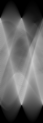
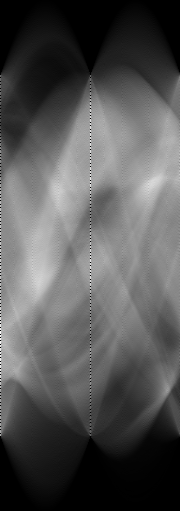
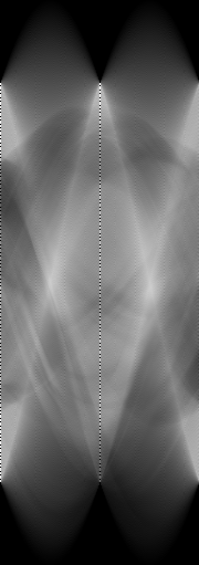
In real CT scans the original image is not known, but the sinogram is. We now use what we have learned so far to try and obtain the original image from a sinogram. We have made three sinograms available on our website, so that you have something to play around with: sinogram_1.png, sinogram_2.png, sinogram_3.png.
p = io.imread('sinogram_1.png')
g = np.transpose(back_projection(p))
100% (180 of 180) |######################| Elapsed Time: 0:01:09 Time: 0:01:09
# Plot the sinogram
plt.subplot(121)
m, n = np.shape(p)
plt.imshow(p, cmap='gray', aspect=n/m, interpolation='nearest')
plt.title(r'Sinogram, $p(s,\theta)$')

# Plot the direct back projection
plt.subplot(122)
plt.imshow(g, cmap='gray', interpolation='nearest')
plt.title('Direct back projection, $g(x,y)$');

Can you see who it is? Let us perform the same filtering as earlier and see if we can get a sharper image.
# Fourier transform of the back projection
spectrum = FFT(g)

# Filter the spectrum
filtered_spectrum = filter_spectrum(spectrum, 'gaussian_highpass', 0.01)

# Inverse Fourier Transform
filtered_g = np.real(IFFT(filtered_spectrum))

# Set all pixels with a negative value to zero
filtered_g = filtered_g*(filtered_g > 0)

# Set all pixels with a value over a certain value to val
val = 4
filtered_g = filtered_g*(filtered_g <= val) + val*(filtered_g > val)

# Visualise the result
plt.imshow(filtered_g, cmap='gray', interpolation='nearest');

Now can you see who it is now? ___
Further work and improvements
- What is the projection slice theorem? How can it be used to argue what the filters look like?
- How can this notebook be generalised to work for an arbitrary $N \times M$ image?
- How can we perform the same calculations on a circular image?
- We have used simple and intuitive algorithms for calculating the sinogram and the direct back projection. Try to find some more sophisticated algorithms. Search for example for radon transformation or check out the TomoPy package.
Sources and further reading
[1] Project description in Norwegian, https://wiki.math.ntnu.no/_media/tma4320/2016v/tomografi.pdf, acquired: 2016-10-21.
[2] A CT scan of an anonymous brain. Provided by Aaron G. Filler, MD, PhD. Image source: https://en.wikipedia.org/wiki/File:Brain_CT_scan.jpg
[3] Shepp, Larry; B. F. Logan (1974). The Fourier Reconstruction of a Head Section. IEEE Transactions on Nuclear Science. NS-21 (3): 21–43. Figure downloaded from https://commons.wikimedia.org/wiki/File:SheppLogan_Phantom.svg [acquired 2 Nov, 2016].