Finite volume methods-2
- Issues:
- Fluxes with variable properties
- See S.V. Patankar "Numerical Heat Transfer and Fluid Flow"
- Grid decoupling
- Fluxes with variable properties
Fluxes with variable properties
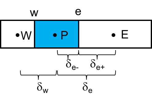
- Consider 1-D, steady state heat conduction on a nonuniform grid.
 $$q_e = -k_e\left(\frac{\partial T}{\partial x}\right)_e,$$$$q_w = -k_w\left(\frac{\partial T}{\partial x}\right)_w.$$
- Consider $q_e$:
- We need $k_e$. How to evaluate it?
Try linear interpolation:
$$\frac{k_E-k_e}{\delta_{e+}} = \frac{k_E-k_P}{\delta_e},$$ $$k_e = fk_P + (1-f)k_E,$$ $$f = \frac{\delta_{e+}}{\delta_e}.$$
Unfortunately, this does not work very well.
- The finite volume method is still conservative since $q_e$ is applied to the energy balance for both the P and E cells.
- But the solution is not physically accurate when applied to systems with variable properties.
Case 1
- Consider the case where cells P and E are different materials.
- Maybe take E as an insulator
- Then $k_E = 0$.
- Expect $q_e = 0$.
- But linear interpolation to evaluate $q_e$ using $k_e$, as shown above, gives the following:
- We expect a temperature profile like the following:
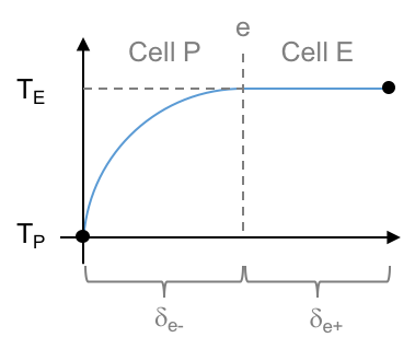
- Notice that no temperature gradient develops in cell E since it is an insulator. This implies zero heat flux.
Case 2
- Now, take a case with $k_E > k_P$.
- We expect the following temperature profile (assuming uniform properties throughout a given control volume):
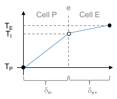 * here, $T_I$ is an intermediate temperature at the cell face e.
If we use a uniform temperature gradient throught the region of interest, then consider the heat fluxes that this graph implies
- Denote the heat flux on the left and right sides of e as $q_{e-}$ and $q_{e+}$, respectively.
- Now, since $k_E\ne k_P$ we have $q_{e-}\ne q_{e+}$.
Hence, using (or implying) the same temperature gradient in both cells (materials) gives different heat fluxes in the two cells when using the respective thermal conductivities.
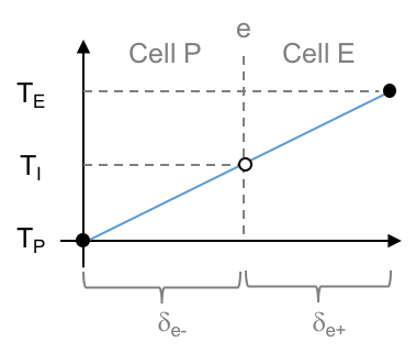
- A linear T profile (same T gradient in both cells) conserves heat flux if the same $k$ is used in both cells.
- That $k$ could be $k_e$ as evaluated by linear interpolation.
- But this gives the unphysical behavior of Case 1.
- And doesn't imply the physical profile of Case 2.
Solution
Find an evaluation of $k_e$, that is physically consistent with heat fluxes through materials of different properties.
That is, find an evaluation of $k_e$ that allows for different temperature gradients to be implied in cells with different conductivities.
Construct $k_e$ by equating fluxes in the two cells (so that energy is conserved):
- Allow for an intermediate temperature $T_I = T_e$.
- Equate the fluxes on the left and right of the interface, and then solve for $T_I$:
- Now equate the flux evaluated over both cells P and E (that is, $q_e$), which is written in terms of $k_e$, and equate this to $q_{e-}$.
- We insert the expression for $T_I$, and then solve for $k_e$:
- This is a harmonic mean instead of an arithmetic mean.
- Use this for finite volume methods with variable $k$, $\mu$, $D$.
- Summary
Results
- Now, for $k_E\rightarrow 0$, $k_e\rightarrow 0$, and $q_e\rightarrow 0$ as it should (unlike the linear interpolation).
- For a case with $k_E\gg k_P$ we have
- This implies that all the change happens in the P cell, with the E cell offering no resistence. Good! This is consistent with the physical situation.
Grid decoupling
- There is a problem with first derivatives.
- Consider cells W, P, E and a convective flux term where $v$ is velocity and $f$ is some variable.
    |---W---|---P---|---E---|
            w       e
- Integrate this over cell P
- Then interpolate to find $(vf)_e$ and $(vf)_w$:
- Note how this totally skips the P cell.
- If we have a $vf$ field as shown below, the first derivative of $vf$ will be zero everywhere and this profile will persist.
|---5---|---3---|---5---|---3---|---5---|
- This can happen in 2D or 3D:
    |-----|-----|-----|
    |  8  |  3  |  8  |
    |-----|-----|-----|
    |  3  |  5  |  3  |
    |-----|-----|-----|
    |  8  |  3  |  8  |
    |-----|-----|-----|
Or, suppose we take a smooth solution and add a checkerboard pattern (from noise, or errors, etc.), this patter could persist, or even grow.
This happens with pressure P in the fluid equations. The $\nabla P$ term gives $P_e-P_w$ hence $(P_E-P_W)/2$.
- Pressure gradients drive velocity, and we'd like pressure to not skip cells. We don't want a pressure checkerboard to be preserved or to grow.
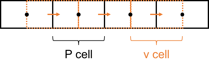
- Remedy: Use a staggered grid.
- Velocity is solved on the orange grid cells (v-cells) and
- Pressure is solved on the black grid cells (P-cells).
- When considering the velocity equation we are using the orange grid (v-cells). Then $dP/dx \rightarrow (P_e-P_w)$, but these values are known directly on the black grid (P-cells) and no interpolation is necessary, and no checkerboarding occurs.
- In 2-D, we have P-cells in the center, u-cells shifted to the left, and v-cells shifted down.
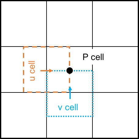
- Normally, scalars such as pressure, temperature, species mass fractions, etc. are evaluated using P-cells, and velocity vectors are on u-cells, v-cells, and w-cells.
- This is convenient for discretization, and numerically very stable.
Grids are called either staggered or collocated.