Denoising Diffusion Probabilistic Model (DDPM)

This notebook focuses on the implementation from scratch of DDPM [1] and is inspired by three great blogs: [2], [3], and [10]

Setup

Diffusion models roughly consist of two parts:

• A predefined forward diffusion process $q(\boldsymbol{x}_t|\boldsymbol{x}_{t-1})$ of our choosing, that gradually adds Gaussian noise to an image until it becomes pure noise.
• A reverse denoising diffusion process $q(\boldsymbol{x}_{t-1}|\boldsymbol{x}_t)$ , approximated by a neural network, which gradually denoises an image starting from pure noise.

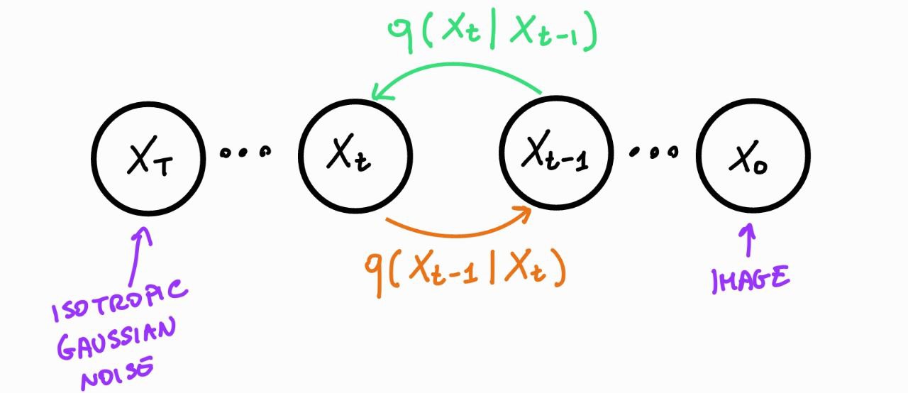
Forward process

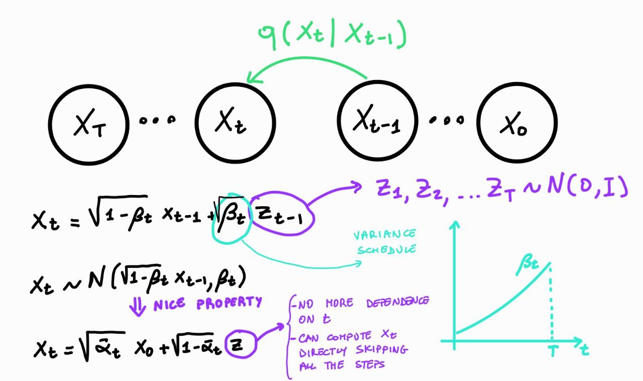
Nice property: Let $\alpha_t = 1 - \beta_t$ and $\bar{\alpha}_t = \prod_{i=1}^t \alpha_i$

\begin{align} \boldsymbol{x}_t & = \sqrt{\alpha_t} \boldsymbol{x}_{t-1} + \sqrt{1 - \alpha_t}\boldsymbol{z}_{t-1} \;\;\; \text{where} \;\boldsymbol{z}_{t-1}, \boldsymbol{z}_{t-2}, \dots, \mathcal{N}(\mathbf{0}, \mathbf{I}).\\ & = \sqrt{\alpha_t} \lbrack \sqrt{\alpha_{t-1}} \boldsymbol{x}_{t-2} + \sqrt{1- \alpha_{t-1}}\boldsymbol{z}_{t-2} \rbrack + \sqrt{1 - \alpha_t}\boldsymbol{z}_{t-1}\\ & = \sqrt{\alpha_t \alpha_{t-1}} \boldsymbol{x}_{t-2} + \sqrt{\alpha_t - \alpha_t \alpha_{t-1}}\boldsymbol{z}_{t-2} + \sqrt{1 - \alpha_t}\boldsymbol{z}_{t-1}\\ & = \sqrt{\alpha_t \alpha_{t-1}} \boldsymbol{x}_{t-2} + \sqrt{1 - \alpha_t \alpha_{t-1}}\boldsymbol{\bar{z}}_{t-2} \;\;\; \text{where} \; \boldsymbol{\bar{z}}_{t-2} \; \text{merges two Gaussians}^1 \\ & = \dots \\ & = \sqrt{\bar{\alpha}_t} \boldsymbol{x}_0 + \sqrt{1 - \bar{\alpha}_t} \boldsymbol{\bar{z}_0} \;\;\; \text{where} \; \boldsymbol{\bar{z}_0} = \boldsymbol{z} \\ q(\boldsymbol{x}_t|\boldsymbol{x}_0) & = \mathcal{N}(\sqrt{\bar{\alpha}_t} \boldsymbol{x}_0, 1 - \bar{\alpha}_t) \end{align}

$^1$ the sum of two Gaussian variables $\boldsymbol{z}_1 \sim \mathcal{N}(\mathbf{0}, \sigma_1^2 \mathbf{I})$ and $\boldsymbol{z}_2 \sim \mathcal{N}(\mathbf{0}, \sigma_2^2 \mathbf{I})$ is a new variable $\bar{\boldsymbol{z}} \sim \mathcal{N}(\mathbf{0}, (\sigma_1^2 + \sigma_2^2) \mathbf{I})$. In our case, $\boldsymbol{z}_{t-1} \sim \mathcal{N}(\mathbf{0}, (1-\alpha_t) \mathbf{I})$ and $\boldsymbol{z}_{t-2} \sim \mathcal{N}(\mathbf{0}, (\alpha_t - \alpha_t \alpha_{t-1}) \mathbf{I})$, so $\boldsymbol{\bar{z}}_{t-2} \sim \mathcal{N}(\mathbf{0}, (1 - \alpha_t \alpha_{t-1}) \mathbf{I})$.

First, we define the scheduler to compute $\beta_t$. The simplest is the linear scheduler, but more advanced schedulers can give better results.

def linear_beta_schedule(timesteps):
    beta_start = 0.0001
    beta_end = 0.02
    return torch.linspace(beta_start, beta_end, timesteps)

timesteps = 200

# compute betas
betas = linear_beta_schedule(timesteps=timesteps)

# compute alphas 
alphas = 1. - betas
alphas_cumprod = torch.cumprod(alphas, axis=0)

# calculations for the forward diffusion q(x_t | x_{t-1})
sqrt_alphas_cumprod = torch.sqrt(alphas_cumprod)
sqrt_one_minus_alphas_cumprod = torch.sqrt(1. - alphas_cumprod)

Let's illustrate how noise is added to a sample image at each time step of the diffusion process.

from PIL import Image
image = Image.open("img/lion_short.png")
image

Next, we resize the image, rescale it in $[-1, 1]$, and convert it to a PyTorch tensor.

from torchvision.transforms import Compose, ToTensor, Lambda, ToPILImage, CenterCrop, Resize

image_size = 128
transform = Compose([
    Resize(image_size),
    ToTensor(), # turn into Numpy array of shape HWC, divide by 255
    Lambda(lambda t: (t * 2) - 1), # [0,1] --> [-1,1]
])

x_start = transform(image).unsqueeze(0)
x_start.shape

torch.Size([1, 3, 128, 128])

We also define the reverse transform, which maps a PyTorch tensor with in $[−1,1]$ back into a PIL image.

reverse_transform = Compose([
     Lambda(lambda t: (t + 1) / 2),
     Lambda(lambda t: t.permute(1, 2, 0)), # CHW to HWC
     Lambda(lambda t: t * 255.),
     Lambda(lambda t: t.numpy().astype(np.uint8)),
     ToPILImage(),
])

reverse_transform(x_start.squeeze())

We can now define the forward diffusion process.

# utility function to extract the appropriate t index for a batch of indices.
# e.g., t=[10,11], x_shape=[b,c,h,w] --> a.shape = [2,1,1,1]
# e.g., t=[7,12,15,20], x_shape=[b,h,w] --> a.shape = [4,1,1]
def extract(a, t, x_shape):
    batch_size = t.shape[0]
    out = a.gather(-1, t.cpu())
    return out.reshape(batch_size, *((1,) * (len(x_shape) - 1))).to(t.device)

# forward diffusion (using the nice property)
def q_sample(x_start, t, noise=None):
    if noise is None:
        noise = torch.randn_like(x_start) # z (it does not depend on t!)
    
    # adjust the shape
    sqrt_alphas_cumprod_t = extract(sqrt_alphas_cumprod, t, x_start.shape)
    sqrt_one_minus_alphas_cumprod_t = extract(
        sqrt_one_minus_alphas_cumprod, t, x_start.shape
    )

    return sqrt_alphas_cumprod_t * x_start + sqrt_one_minus_alphas_cumprod_t * noise

Let's test on a specific time step, $t=20$:

def get_noisy_image(x_start, t):
  
  x_noisy = q_sample(x_start, t=t) # add noise
  noisy_image = reverse_transform(x_noisy.squeeze()) # turn back into PIL image

  return noisy_image

t = torch.tensor([19])
get_noisy_image(x_start[0], t)

plot_seq([get_noisy_image(x_start, torch.tensor([t])) for t in [1, 50, 100, 150, 199]])

Backward process

• If $\beta_t$ is small enough, $q(\boldsymbol{x}_{t-1}|\boldsymbol{x}_t)$ will be a Gaussian $\mathcal{N}\big(\tilde{\mu}(\boldsymbol{x}_t), \tilde{\sigma}(\boldsymbol{x}_t)\big)$
• However, we cannot compute $\tilde{\mu}(\boldsymbol{x}_t)$ and $\tilde{\sigma}(\boldsymbol{x}_t)$ analytically, because requires knowing the true data distribution $p(\boldsymbol{x})$

$$ q(\boldsymbol{x}_{t-1}|\boldsymbol{x}_t)q(\boldsymbol{x}_{t-2}|\boldsymbol{x}_{t-1})\dots \rightarrow p(\boldsymbol{x}_0)$$

• We can use a NN to learn $\tilde{\mu}(\boldsymbol{x}_t)$ and $\tilde{\sigma}(\boldsymbol{x}_t)$

Simplification

Represent $\tilde{\sigma}(\boldsymbol{x}_t)$ with a time dependent constant $\tilde{\beta}_t$

Manipulation

Condition on $\boldsymbol{x}_0$ and obtain $q(\boldsymbol{x}_{t-1}|\boldsymbol{x}_t$ , $\boldsymbol{x}_0$ $)$ $ = \mathcal{N} \big( $ $\tilde{\mu}(\boldsymbol{x}_t, \boldsymbol{x}_0)$ , $\tilde{\beta}_t$ $\big) = \mathcal{N} \big( $ $\tilde{\mu}_t$ , $\tilde{\beta}_t$ $\big)$

where

$\tilde{\beta}_t = \frac{1 - \bar \alpha_{t-1}}{1 - \bar \alpha_{t}} \beta_t$

and

$\tilde{\mu}_t = \frac{1}{\sqrt{\alpha_t}} \Big(\boldsymbol{x}_t - \frac{\beta_t}{\sqrt{1 - \bar{\alpha}_t}}$ $\boldsymbol{\tilde z}_t$ $\Big)$

NN Model

• Take a look at $\tilde{\beta}_t = \frac{1 - \bar \alpha_{t-1}}{1 - \bar \alpha_{t}} \beta_t$

and $\tilde{\mu}_t = \frac{1}{\sqrt{\alpha_t}} \Big(\boldsymbol{x}_t - \frac{\beta_t}{\sqrt{1 - \bar{\alpha}_t}}$ $\boldsymbol{\tilde z}_t$ $\Big)$ - The only thing we do not know is $\boldsymbol{\tilde z}_t$ . - We approximate $\boldsymbol{\tilde z}_t$ with a NN.

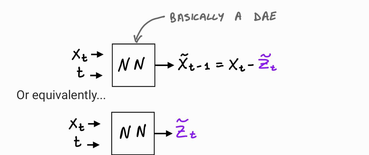
As NN, we use a Unet.

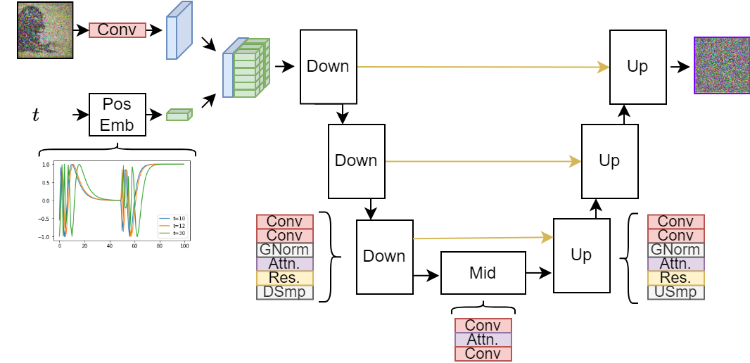
# Let's check the input and output of the U-net
from scripts.unet import Unet

temp_model = Unet(
    dim=image_size,
    channels=3,
    dim_mults=(1, 2, 4,)
)

with torch.no_grad():
    out = temp_model(x_start, torch.tensor([40]))
    
print(f"input shape: {x_start.shape}, output shape: { out.shape}")

input shape: torch.Size([1, 3, 128, 128]), output shape: torch.Size([1, 3, 128, 128])

Loss

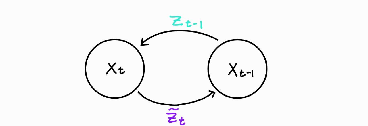
• Loss: $ \| $ $\boldsymbol{ z}_{t-1}$ - $\boldsymbol{\tilde z}_{t}$ $\|_1 = \| $ $\boldsymbol{ z}_{t-1}$ - NN$(\boldsymbol{x}_t, t)$ $\|_1$
• $\boldsymbol{ z}_{t-1}$ is the noise used to compute $\boldsymbol{x}_t$ in the forward process
• Remember that to compute $\boldsymbol{x}_t$ we dropped the time index on $\boldsymbol{z}$ (nice property):

$$ \boldsymbol{x}_t = \sqrt{\bar \alpha_t} \boldsymbol{x}_0 + \sqrt{1 - \bar \alpha_t} \boldsymbol{z} $$

• Simply, we can sample $\boldsymbol{z}$ , compute $\boldsymbol{x}_t$, and recover $\boldsymbol{z}$ with the $NN$

Training

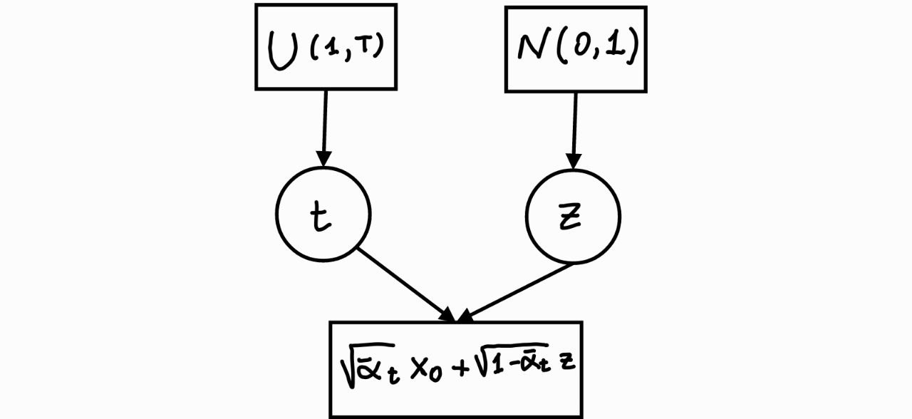
repeat

• Sample an image from the training data
  • $\boldsymbol{x}_0 \sim p(\boldsymbol{x}_0)$
• Sample $\boldsymbol{ z}$ and $t$ randomly
  • $t \sim \mathcal{U}([1, T])$
  • $\boldsymbol{ z}$ $\sim \mathcal{N}(\boldsymbol{0}, \boldsymbol{I})$
• Take gradient descent step on

$ \nabla_\theta \|$ $\boldsymbol{ z}$ -

NN$( \sqrt{\bar \alpha_t} \boldsymbol{x}_0 + \sqrt{1 - \bar \alpha_t}$ $\boldsymbol{z}$ $)$ $\|_1 $

until converged

def p_losses(denoise_model, x_start, t, loss_type="huber"):

    # random sample z    
    noise = torch.randn_like(x_start)
    
    # compute x_t
    x_noisy = q_sample(x_start=x_start, t=t, noise=noise)
    
    # recover z from x_t with the NN
    predicted_noise = denoise_model(x_noisy, t)

    if loss_type == 'l1':
        loss = F.l1_loss(noise, predicted_noise)
    elif loss_type == 'l2':
        loss = F.mse_loss(noise, predicted_noise)
    elif loss_type == "huber":
        loss = F.smooth_l1_loss(noise, predicted_noise)
    else:
        raise NotImplementedError()

    return loss

Sampling

We said that $\boldsymbol{x}_{t-1} \sim \mathcal{N} \big( $ $\tilde{\mu}_t$ , $\tilde{\beta}_t$ $\big)$ where

$\tilde{\beta}_t = \frac{1 - \bar \alpha_{t-1}}{1 - \bar \alpha_{t}} \beta_t$ and $\tilde{\mu}_t = \frac{1}{\sqrt{\alpha_t}} \Big(\boldsymbol{x}_t - \frac{\beta_t}{\sqrt{1 - \bar{\alpha}_t}}$ $\boldsymbol{\tilde z}_t$ $\Big)$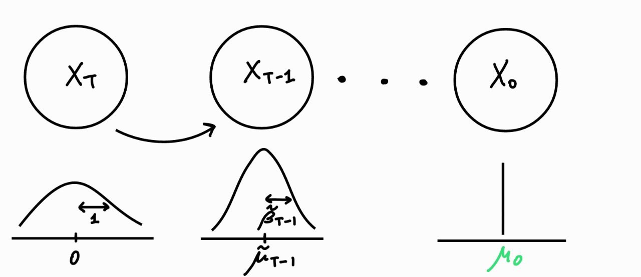

Sampling algorithm

$\boldsymbol{x}_T \sim \mathcal{N}(\boldsymbol{0}, \boldsymbol{I})$

for $t=T-1, \dots, 0$ do

• $\boldsymbol{z} \sim \mathcal{N}(\boldsymbol{0}, \boldsymbol{I})$ if $t > 1$ else $\boldsymbol{z}=0$
• $\boldsymbol{x}_{t-1} = \frac{1}{\sqrt{\alpha_t}} \big( \boldsymbol{x}_{t} - \frac{\beta_t}{\sqrt{1 - \bar{ \alpha}_t}}$ NN$(\boldsymbol{x}_t, t)$ $\big) + \tilde \beta_t \boldsymbol{z}$

return $\boldsymbol{x}_{0} = \mu_0$

# calculations for posterior q(x_{t-1} | x_t, x_0) = q(x_{t-1} | t, x_0)
sqrt_recip_alphas = torch.sqrt(1.0 / alphas)
alphas_cumprod_prev = F.pad(alphas_cumprod[:-1], (1, 0), value=1.0)
posterior_variance = betas * (1. - alphas_cumprod_prev) / (1. - alphas_cumprod) # β_t
 
@torch.no_grad()
def p_sample(model, x, t, t_index):
     
    # adjust shapes
    betas_t = extract(betas, t, x.shape)
    sqrt_one_minus_alphas_cumprod_t = extract(
        sqrt_one_minus_alphas_cumprod, t, x.shape
    )
    sqrt_recip_alphas_t = extract(sqrt_recip_alphas, t, x.shape)
    
    # Use the NN to predict the mean
    model_mean = sqrt_recip_alphas_t * (
        x - betas_t * model(x, t) / sqrt_one_minus_alphas_cumprod_t)

    # Draw the next sample
    if t_index == 0:
        return model_mean
    else:
        posterior_variance_t = extract(posterior_variance, t, x.shape)  # beta_t
        noise = torch.randn_like(x)                                     # z
        return model_mean + torch.sqrt(posterior_variance_t) * noise    # x_{t-1}

# Sampling loop
@torch.no_grad()
def p_sample_loop(model, shape):
    device = next(model.parameters()).device

    # start from pure noise (for each example in the batch)
    img = torch.randn(shape, device=device)
    imgs = []

    for i in tqdm(reversed(range(0, timesteps)), desc='sampling loop time step', total=timesteps):
        img = p_sample(model, img, torch.full((shape[0],), i, device=device, dtype=torch.long), i)
        imgs.append(img)
    return imgs

@torch.no_grad()
def sample(model, image_size, batch_size=16, channels=3):
    return p_sample_loop(model, shape=(batch_size, channels, image_size, image_size))

Train the model on Fashion MNIST

from datasets import load_dataset

dataset = load_dataset("fashion_mnist")
image_size = 28
channels = 1
batch_size = 128

Downloading readme:   0%|          | 0.00/9.02k [00:00<?, ?B/s]

Downloading data: 100%|██████████████████████████████████████████████████████████████████████████████████| 30.9M/30.9M [00:01<00:00, 22.0MB/s]
Downloading data: 100%|██████████████████████████████████████████████████████████████████████████████████| 5.18M/5.18M [00:00<00:00, 9.24MB/s]

Generating train split:   0%|          | 0/60000 [00:00<?, ? examples/s]

Generating test split:   0%|          | 0/10000 [00:00<?, ? examples/s]

Next, we define some basic image preprocessing on-the-fly: random horizontal flips, converstion to tensor, and rescaling in the $[-1,1]$ range.

We use with_transform to apply the transformations to the elements in the dataset.

from torchvision import transforms
from torch.utils.data import DataLoader

# define image transformations (e.g. using torchvision)
transform = Compose([
            transforms.RandomHorizontalFlip(),
            transforms.ToTensor(),
            transforms.Lambda(lambda t: (t * 2) - 1)
])

# define function
def transforms(examples):
   examples["pixel_values"] = [transform(image.convert("L")) for image in examples["image"]]
   del examples["image"]

   return examples

transformed_dataset = dataset.with_transform(transforms).remove_columns("label")

# create dataloader
dataloader = DataLoader(transformed_dataset["train"], batch_size=batch_size, shuffle=True)

from torch.optim import Adam

device = "cuda" if torch.cuda.is_available() else "cpu"

model = Unet(
    dim=image_size,
    channels=channels,
    dim_mults=(1, 2, 4,)
)
model.to(device)

optimizer = Adam(model.parameters(), lr=1e-3)

from torchvision.utils import save_image

epochs = 10

for epoch in range(epochs):
    for step, batch in enumerate(dataloader):
      optimizer.zero_grad()

      # x0
      batch_size = batch["pixel_values"].shape[0]
      batch = batch["pixel_values"].to(device)

      # sample t from U(0,T)
      t = torch.randint(0, timesteps, (batch_size,), device=device).long()
      
      loss = p_losses(model, batch, t)

      if step % 100 == 0:
        print(f"Epoch: {epoch}, step: {step} -- Loss: {loss.item():.3f}")

      loss.backward()
      optimizer.step() 

Epoch: 0, step: 0 -- Loss: 0.472
Epoch: 0, step: 100 -- Loss: 0.145
Epoch: 0, step: 200 -- Loss: 0.090
Epoch: 0, step: 300 -- Loss: 0.072
Epoch: 0, step: 400 -- Loss: 0.064
Epoch: 1, step: 0 -- Loss: 0.061
Epoch: 1, step: 100 -- Loss: 0.059
Epoch: 1, step: 200 -- Loss: 0.063
Epoch: 1, step: 300 -- Loss: 0.060
Epoch: 1, step: 400 -- Loss: 0.047
Epoch: 2, step: 0 -- Loss: 0.047
Epoch: 2, step: 100 -- Loss: 0.058
Epoch: 2, step: 200 -- Loss: 0.047
Epoch: 2, step: 300 -- Loss: 0.051
Epoch: 2, step: 400 -- Loss: 0.046
Epoch: 3, step: 0 -- Loss: 0.051
Epoch: 3, step: 100 -- Loss: 0.045
Epoch: 3, step: 200 -- Loss: 0.042
Epoch: 3, step: 300 -- Loss: 0.046
Epoch: 3, step: 400 -- Loss: 0.048
Epoch: 4, step: 0 -- Loss: 0.043
Epoch: 4, step: 100 -- Loss: 0.051
Epoch: 4, step: 200 -- Loss: 0.042
Epoch: 4, step: 300 -- Loss: 0.046
Epoch: 4, step: 400 -- Loss: 0.045
Epoch: 5, step: 0 -- Loss: 0.050
Epoch: 5, step: 100 -- Loss: 0.045
Epoch: 5, step: 200 -- Loss: 0.045
Epoch: 5, step: 300 -- Loss: 0.047
Epoch: 5, step: 400 -- Loss: 0.044
Epoch: 6, step: 0 -- Loss: 0.042
Epoch: 6, step: 100 -- Loss: 0.042
Epoch: 6, step: 200 -- Loss: 0.044
Epoch: 6, step: 300 -- Loss: 0.041
Epoch: 6, step: 400 -- Loss: 0.040
Epoch: 7, step: 0 -- Loss: 0.046
Epoch: 7, step: 100 -- Loss: 0.039
Epoch: 7, step: 200 -- Loss: 0.044
Epoch: 7, step: 300 -- Loss: 0.046
Epoch: 7, step: 400 -- Loss: 0.041
Epoch: 8, step: 0 -- Loss: 0.048
Epoch: 8, step: 100 -- Loss: 0.045
Epoch: 8, step: 200 -- Loss: 0.042
Epoch: 8, step: 300 -- Loss: 0.048
Epoch: 8, step: 400 -- Loss: 0.040
Epoch: 9, step: 0 -- Loss: 0.047
Epoch: 9, step: 100 -- Loss: 0.045
Epoch: 9, step: 200 -- Loss: 0.041
Epoch: 9, step: 300 -- Loss: 0.035
Epoch: 9, step: 400 -- Loss: 0.050

Inference

Once trained, we can sample from the model using sample the function defined above:

# Generate 64 images
samples = sample(model, image_size=image_size, batch_size=64, channels=channels)

# Get the last sample and normalize it in [0,1]
last_sample = (samples[-1] - samples[-1].min())/(samples[-1].max()-samples[-1].min())

grid_img = torchvision.utils.make_grid(last_sample, nrow=16)
%matplotlib inline
plt.figure(figsize = (20,10))
plt.imshow(grid_img.permute(1, 2, 0).cpu().numpy(), cmap='gray');

sampling loop time step:   0%|          | 0/200 [00:00<?, ?it/s]

Next steps

• Sample generation can be conditioned on inputs such as text (text2img) and images (img2img) [4].
• Besides the mean, learning the standard deviation $\tilde{\sigma}(\boldsymbol{x}_t)$ of the conditional distribution helps in improving performance [5].
• More advanced noise scheduler than the linear one can give better performance and decrease inference time [6]
• Diffusion in the pixel space is slow. Latent diffusion, in the embedding space, can speed-up inference time greatly [7]

Conditioned generation with diffusion guidance

Score-Based Generative Models

• Different from DDPM, yet equivalent in nature, are the score-based methods [8]
• Score-based generative models and DDPM are different perspectives of the same model family
• In this perspective, the desnoising process corresponds to taking steps in the direction of the score function

$$\nabla_x \log{p(x)}$$

i.e., the direction where the log-likelihood increases the most

• In the process, noise is added to avoid getting stuck between the modes of the distribution
• This is called Stochastic Gradient Langevin Dynamics (SGLD)

Conditional models

• In conditional models, we want to model $p(x|y)$
• In the score-based perspective, it means following during diffusion the score function: $\nabla_x \log{p(x|y)}$
• By applying Bayes' rule

$$ p(x|y) = \frac{p(y|x)p(x)}{p(y)}$$

that gives us $$ \nabla_x \log{p(x|y)} = \nabla_x \log{p(y|x)} + \nabla_x \log{p(x)} - \nabla_x \log{p(y)} = \nabla_x \log{p(y|x)} + \nabla_x \log{p(x)}$$

• Notice that $p(y|x)$ is exactly what an image classifier tries to fit
• If the image classifier is a neural net, it is easy to compute $\nabla_x \log{p(y|x)}$

• We can give different contributions to the score function and the classfier

$$\nabla_x \log{p_\gamma(x|y)} = \nabla_x \log{p(x)} + \gamma \nabla_x \log{p(y|x)},$$

where $\gamma$ is the guidance scale [9]

• The larger $\gamma$, the larger is the influence of the conditioning signal
• Reverting the gradient and the logarithm operations, we see that $p_\gamma(x|y) \propto p(x)p(y|x)^\gamma$
• When $\gamma >1$, this sharpens the distribution and shift probability mass towards the values $x$ that are most likely associated with label $y$

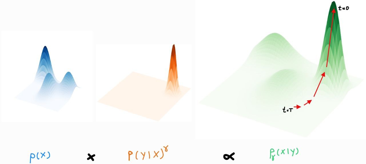
• ⚠️ Important: the diffusion model is trained as before and only at inference time is conditioned by a (pre-trained) classifier
• Similar to train a powerful unconditional NLP model and adapt it to downstream tasks via few-shot learning

Limitations

❌ Pre-trained classifiers cannot deal with noise

• The classifier used for guidance needs to cope with high noise to provide a useful signal through the sampling process
• This usually requires training the classifier specifically for the purpose of guidance
• At that point, it might be easier to train a traditional conditional generative model end-to-end...

❌ Classifiers take shortcuts

• Most of the information in the input $x$ is not accounted in predicting $y$
• As result, taking the gradient of the classifier w.r.t. its input can yield arbitrary directions in input space

Classifier-free guidance (cfg)

• We said that $\nabla_x \log{p(x|y)} = \nabla_x \log{p(y|x)} + \nabla_x \log{p(x)}$
• Now, let's express the conditioning term as a function of the conditional and unconditional score functions, both of which our diffusion model provides

$$ \nabla_x \log{p(y|x)} = \nabla_x \log{p(x|y)} - \nabla_x \log{p(x)}$$

• Then, we substitute this into the formula for classifier guidance:

$$ \nabla_x \log{p_\gamma(x|y)} = \nabla_x \log{p(x)} + \gamma \big[ \nabla_x \log{p(x|y)} - \nabla_x \log{p(x)} \big]$$

• We expressed the conditional score function as a combination of the conditional and the unconditional score function itself
• We no longer need a classifier!

• cfg is implemented by removing the conditioning signal 10-20% of times while training (conditioning dropout)[11]
• In practice, one replaces $y$ with a special input value representing the absence of conditioning information (e.g., "")
• The resulting model is now able to function both as a conditional model $p(x|y)$ and as an unconditional model $p(x)$, depending on whether the conditioning signal is provided

Example: "A stained glass window of a panda eating bamboo." with classifier guidance (left) and with cfg (right)

Why cfg is better than classifier guidance?

• cfg replaces the guidance from a standard classifier $\nabla_x \log{p(y|x)}$ with a "classifier" built from a generative model $\nabla_x \log{p(x|y)} - \nabla_x \log{p(x)}$.
• Standard classifiers can take shortcuts and ignore most of the input $x$ while still obtaining competitive classification results
• Instead, generative models are forced to consider the whole data distribution, making the gradient much more robust
• In addtion, we only have to train a single (generative) model, and conditioning dropout is trivial to implement

Limitation:

• cfg dramatically improves adherence to the conditioning signal and the overall sample quality at the cost of diversity
• This is a tipycal trade-off in generative models

References

[1] Ho, J., Jain, A., Abbeel, P., (2020). Denoising diffusion probabilistic models. Advances in Neural Information Processing Systems.

[2] Rogge, N., Rasul, K., (2022). The Annotated Diffusion Model.

[3] Dieleman, S., (2022). Guidance: a cheat code for diffusion models.

[4] Ramesh, A., Dhariwal, P., Nichol, A., Chu, C., & Chen, M. (2022). Hierarchical text-conditional image generation with clip latents.

[5] Nichol, A. Q., & Dhariwal, P. (2021). Improved denoising diffusion probabilistic models. In International Conference on Machine Learning.

[6] Song, J., Meng, C., & Ermon, S. (2020). Denoising diffusion implicit models.

[7] Rombach, R., Blattmann, A., Lorenz, D., Esser, P., & Ommer, B. (2022). High-resolution image synthesis with latent diffusion models. In Proceedings of the IEEE/CVF Conference on Computer Vision and Pattern Recognition.

[8] Song, Y., Sohl-Dickstein, J., Kingma, D. P., Kumar, A., Ermon, S., & Poole, B. (2021). Score-Based Generative Modeling through Stochastic Differential Equations. International Conference on Learning Representations.

[9] Dhariwal, P., & Nichol, A. (2021). Diffusion models beat gans on image synthesis. Advances in Neural Information Processing Systems.

[10] Weng, L., (2021). What are diffusion models?

[11] Nichol, A., Dhariwal, P., Ramesh, A., Shyam, P., Mishkin, P., McGrew, B., ... & Chen, M. (2021). Glide: Towards photorealistic image generation and editing with text-guided diffusion models.