%matplotlib inline
import matplotlib.pyplot as plt
import numpy as np
import skimage as ski
from skimage.morphology import disk
import scipy.ndimage as ndimage

A typical processing chain

plt.figure(figsize=[15,6]);
plt.subplot(1,3,1);plt.imshow(np.random.normal(0,1,[100,100])); plt.title('Gaussian');plt.axis('off');
plt.subplot(1,3,2);plt.imshow(0.90<np.random.uniform(0,1,size=[100,100]),cmap='gray'); plt.title("Salt and pepper"),plt.axis('off');
plt.subplot(1,3,3);plt.imshow(ski.filters.gaussian(np.random.normal(0,1,size=[100,100]),sigma=1),cmap='gray'); plt.title("Structured"),plt.axis('off');
plt.tight_layout()
from scipy.stats import norm
rv = norm(loc = -1., scale = 1.0);rv1 = norm(loc = 0., scale = 2.0); rv2 = norm(loc = 2., scale = 3.0)
x = np.arange(-10, 10, .1)

#plot the pdfs of these normal distributions
plt.plot(x, rv.pdf(x),label='$\mu$=-1, $\sigma$=1')
plt.plot(x, rv1.pdf(x),label='$\mu$=0, $\sigma$=2')
plt.plot(x, rv2.pdf(x),label='$\mu$=2, $\sigma$=3')
plt.legend()
from scipy.stats import poisson
mu=3
fig, ax = plt.subplots(1, 1)
x = np.arange(poisson.ppf(0.01, mu),              poisson.ppf(0.999, mu))
ax.plot(x, poisson.pmf(x, mu), 'bo', ms=8, label='poisson pmf')
ax.vlines(x, 0, poisson.pmf(x, mu), colors='b', lw=5, alpha=0.5)
plt.figure(figsize=[15,8])
x=np.linspace(0,2*np.pi,100);
y=10*np.sin(x)+11; ng=np.random.normal(0,1,size=len(x)); npoi = np.random.poisson(y);
plt.subplot(2,2,1); plt.plot(x,y+ng);plt.plot(x,y); plt.axis('off');plt.title('Gaussian'); plt.subplot(2,2,3);plt.plot(x,ng);plt.axis('off');
plt.subplot(2,2,2); plt.plot(x,npoi);plt.plot(x,y); plt.axis('off');plt.title('Poisson'); plt.subplot(2,2,4);plt.plot(x,npoi-y);plt.axis('off');
Noise models - Salt'n'pepper noise
- A type of outlier noise
- Noise frequency described as probability of outlier
- Can be additive, multiplicative, and independent replacement
Example model
$sp(x)=\left\{\begin{array}{ll} -1 & x\leq\lambda_1\\ 0 & \lambda_1< x \leq \lambda_2\\ 1 & \lambda_2<x \end{array}\right.\qquad \begin{array}{l}x\in\mathcal{U}(0,1)\\\lambda_1<\lambda_2\\ \lambda_1+\lambda_2 = \mbox{noise fraction} \end{array}$
Salt'n'pepper examples
def snp(dims,Pblack,Pwhite) : # Noise model function
    uni=np.random.uniform(0,1,dims)
    img=(Pwhite<uni).astype(float)-(uni<Pblack).astype(float)
    return img
img10_90=snp([100,100],0.1,0.9); img5_95=snp([100,100],0.05,0.95);img1_99=snp([100,100],0.01,0.99)
plt.figure(figsize=[15,5])
plt.subplot(1,3,1); plt.imshow(img1_99,cmap='gray'); plt.title('$\lambda_1$=1% and $\lambda_2$=99%',fontsize=16); plt.axis('off');
plt.subplot(1,3,2); plt.imshow(img5_95,cmap='gray'); plt.title('$\lambda_1$=5% and $\lambda_2$=95%',fontsize=16); plt.axis('off');
plt.subplot(1,3,3); plt.imshow(img10_90,cmap='gray'); plt.title('$\lambda_1$=10% and $\lambda_2$=90%',fontsize=16); plt.axis('off');
Signal to noise ratio for Poisson noise
- For a Poisson distribution the SNR is :
$SNR \sim \sqrt{N}$
- $N$ is the number of particles $\sim$ exposure time
exptime=np.array([50,100,200,500,1000,2000,5000,10000])
snr = np.array([ 8.45949767, 11.40011621, 16.38118766, 21.12056507, 31.09116641,40.65323123, 55.60833117, 68.21108979]);
marker_style = dict(color='cornflowerblue', linestyle='-', marker='o',markersize=10, markerfacecoloralt='gray');
plt.figure(figsize=(15,5))
plt.subplot(1,3,2);plt.plot(exptime/1000,snr, **marker_style);plt.xlabel('Exposure time [s]');plt.ylabel('SNR [1]')
img50ms=plt.imread('ext-figures/lecture03/tower_50ms.png'); img10000ms=plt.imread('ext-figures/lecture03/tower_10000ms.png');
plt.subplot(1,3,1);plt.imshow(img50ms); plt.subplot(1,3,3); plt.imshow(img10000ms);
Useful python functions
Random number generators [numpy.random]
Generate an $m \times n$ random fields with different distributions:
- Gauss
np.random.normal(mu,sigma, size=[rows,cols]) - Uniform
np.random.uniform(low,high,size=[rows,cols]) - Poisson ```np.random.poisson(lambda, size=[rows,cols])
Statistics
np.mean(f),np.var(f),np.std(f)Computes the mean, variance, and standard deviation of an image $f$.np.min(f),np.max(f)Finds minimum and maximum values in $f$.np.median(f),np.rank()Selects different values from the sorted data.
Basic filtering
Filter characteristics
Filters are characterized by the type of information they suppress


Basic filters
Linear filters
Computed using the convolution operation
$$g(x)=h*f(x)=\int_{\Omega}f(x-\tau) h(\tau) d\tau$$where
- $f$ is the image
- $h$ is the convolution kernel of the filter

Low-pass filter kernels
| Mean or Box filter | Gauss filter |
| All weights have the same value. | $$G=\exp{-\frac{x^2+y^2}{2\,\sigma^2}}$$ |
|
Example: $$B=\frac{1}{25}\cdot\begin{array}{|c|c|c|c|c|} \hline 1 & 1 & 1 & 1& 1\\ \hline 1 & 1 & 1 & 1& 1\\ \hline 1 & 1 & 1 & 1& 1\\ \hline 1 & 1 & 1 & 1& 1\\ \hline 1 & 1 & 1 & 1& 1\\ \hline \end{array} $$ |
Example:  |
Different SNR using a Gauss filter
img = plt.imread('ext-figures/lecture03/input_orig.png');
noise = np.random.normal(0,1,size=img.shape); snr10=img+0.1*noise; snr5=img+0.2*noise; snr2=img+0.5*noise;plt.figure(figsize=[15,12])
plt.subplot(3,4,1); plt.imshow(img); plt.axis('off');plt.title('No noise'); plt.subplot(3,4,2); plt.imshow(snr10); plt.title('SNR=10'); plt.axis('off');plt.subplot(3,4,3); plt.imshow(snr5); plt.title('SNR=5'); plt.axis('off');plt.subplot(3,4,4); plt.imshow(snr2); plt.title('SNR=2'); plt.axis('off');
plt.subplot(3,4,5); plt.imshow(ski.filters.gaussian(img,sigma=1)); plt.title('Gaussian $\sigma$=1'); plt.axis('off');plt.subplot(3,4,6); plt.imshow(ski.filters.gaussian(snr10,sigma=1));  plt.axis('off');plt.subplot(3,4,7); plt.imshow(ski.filters.gaussian(snr5,sigma=1));  plt.axis('off');plt.subplot(3,4,8); plt.imshow(ski.filters.gaussian(snr2,sigma=1)); plt.axis('off');
plt.subplot(3,4,9); plt.imshow(ski.filters.gaussian(img,sigma=3)); plt.title('Gaussian $\sigma$=3'); plt.axis('off');plt.subplot(3,4,10); plt.imshow(ski.filters.gaussian(snr10,sigma=3));  plt.axis('off');plt.subplot(3,4,11); plt.imshow(ski.filters.gaussian(snr5,sigma=3));  plt.axis('off');plt.subplot(3,4,12); plt.imshow(ski.filters.gaussian(snr2,sigma=3)); plt.axis('off');
How is the convolution computed

Euclidean separability
The asociative and commutative laws apply to convoution
$$(a * b)*c=a*(b*c) \quad \mbox{ and } \quad a * b = b * a $$A convolution kernel is called separable if it can be split in two or more parts:
$$\begin{array}{|c|c|c|} \hline \cdot & \cdot & \cdot\\ \hline \cdot & \cdot & \cdot\\ \hline \cdot & \cdot& \cdot\\ \hline \end{array}= \begin{array}{|c|} \hline \cdot \\ \hline \cdot \\ \hline \cdot \\ \hline \end{array} * \begin{array}{|c|c|c|} \hline \cdot & \cdot & \cdot\\ \hline \end{array}$$ $$\exp{-\frac{x^2+y^2}{2\,\sigma^2}}=\exp{-\frac{x^2}{2\,\sigma^2}}*\exp{-\frac{y^2}{2\,\sigma^2}}$$Gain
Separability reduces the number of computations $\rightarrow$ faster processing
- 3$\times$3 $\rightarrow$ 9 mult and 8 add $\Leftrightarrow$ 6 mult and 4 add
- 3$\times$3$\times$3 $\rightarrow$ 27 mult and 26 add $\Leftrightarrow$ 9 mult and 6 add
The median filter

Comparing filters for different noise types
img = plt.imread('ext-figures/lecture03/grasshopper.png'); noise=img+np.random.normal(0,0.1,size=img.shape); spots=img+0.2*snp(img.shape,0,0.8); noise=(noise-noise.min())/(noise.max()-noise.min());spots=(spots-spots.min())/(spots.max()-spots.min());
plt.figure(figsize=[15,10]);
plt.subplot(2,3,1); plt.imshow(spots); plt.title('Spots'); plt.axis('off');
plt.subplot(2,3,2); plt.imshow(ski.filters.gaussian(spots,sigma=1)); plt.title('Gauss filter'); plt.axis('off');
plt.subplot(2,3,3); plt.imshow(ski.filters.median(spots,disk(3))); plt.title('Median'); plt.axis('off');

plt.subplot(2,3,4); plt.imshow(noise); plt.title('Gaussian noise'); plt.axis('off');
plt.subplot(2,3,5); plt.imshow(ski.filters.gaussian(noise,sigma=1)); plt.title('Gauss filter'); plt.axis('off');
plt.subplot(2,3,6); plt.imshow(ski.filters.median(noise,disk(3))); plt.title('Median'); plt.axis('off');
Filter example: Spot cleaning
| Problem | Example | Possible solutions |
|---|---|---|
|
 |
|


High-pass filters
High-pass filters enhance rapid changes $\rightarrow$ ideal for edge detection
Typical high-pass filters:
Gradients
$$\frac{\partial}{\partial\,x}=\frac{1}{2}\cdot\begin{array}{|c|c|} \hline -1 & 1\\ \hline \end{array}\qquad \frac{\partial}{\partial\,x}=\frac{1}{32}\cdot\begin{array}{|c|c|c|} \hline -3 & 0 & 3\\ \hline -10 & 0 & 10\\ \hline -3 & 0 & 3\\ \hline \end{array} $$Laplacian
$$ \bigtriangleup=\frac{1}{2}\cdot\begin{array}{|c|c|c|} \hline 1 & 2 & 1\\ \hline 2 & -12 & 2\\ \hline 1 & 2 & 1\\ \hline \end{array} $$Sobel
$$ G=|\nabla f|=\sqrt{\left(\frac{\partial}{\partial\,x}f\right)^2 + \left(\frac{\partial}{\partial\,y}f\right)^2} $$Gradient example
Vertical edges
$\frac{\partial}{\partial x}=\frac{1}{32}\cdot\begin{array}{|c|c|c|} \hline -3 & 0 & 3\\ \hline -10 & 0 & 10\\ \hline -3 & 0 & 3\\ \hline \end{array}$
Horizontal egdges
$\frac{\partial}{\partial\,y}=\frac{1}{32}\cdot\begin{array}{|c|c|c|} \hline -3 & -10 & -3\\ \hline 0 & 0 & 0\\ \hline 3 & 10 & 3\\ \hline \end{array}$
img=plt.imread('ext-figures/lecture03/orig.png')
k = np.array([[-3,-10,-3],[0,0,0],[3,10,3]]);
plt.figure(figsize=[15,8])
plt.subplot(1,3,1); plt.imshow(img);plt.title('Original');
plt.subplot(1,3,2); plt.imshow(ndimage.convolve(img,np.transpose(k)));plt.title('$\partial / \partial x$');
plt.subplot(1,3,3); plt.imshow(ndimage.convolve(img,k));plt.title('$\partial / \partial y$');
Edge detection examples
img=plt.imread('ext-figures/lecture03/orig.png');
plt.figure(figsize=[15,6])
plt.subplot(1,2,1);plt.imshow(ski.filters.laplace(img),clim=[-0.08,0.08]); plt.title('Laplacian'); plt.colorbar();
plt.subplot(1,2,2);plt.imshow(ski.filters.sobel(img)); plt.title('Sobel');  plt.colorbar();
Relevance of filters to machine learning

The Fourier transform
Transform
$$G(\xi_1,\xi_2)=\mathcal{F}\{g\}=\int_{-\infty}^{\infty}\int_{-\infty}^{\infty} g(x,y) \exp{-i(\xi_1\,x+\xi_2\,y)}\,dx\,dy$$Inverse
$$ g(x,y)=\mathcal{F}^{-1}\{G\}=\frac{1}{(2\,\pi)^2}\int_{-\infty}^{\infty}\int_{-\infty}^{\infty} G(\omega) \exp{i(\xi_1\,x+\xi_2\,y)}\,d\xi_1 \,d\xi_2$$FFT (Fast Fourier Transform)
In practice - you never see the transform equations. The Fast Fourier Transform algorithm is available in numerical libraries and tools.
x = np.linspace(0,50,100); s0=np.sin(0.5*x); s1=np.sin(2*x);
plt.figure(figsize=[15,5])
plt.subplot(2,3,1);plt.plot(x,s0); plt.axis('off');plt.title('$s_0$');plt.subplot(2,3,4);plt.plot(np.abs(np.fft.fftshift(np.fft.fft(s0))));plt.axis('off');
plt.subplot(2,3,2);plt.plot(x,s1); plt.axis('off');plt.title('$s_1$');plt.subplot(2,3,5);plt.plot(np.abs(np.fft.fftshift(np.fft.fft(s1))));plt.axis('off');
plt.subplot(2,3,3);plt.plot(x,s0+s1); plt.axis('off');plt.title('$s_0+s_1$');plt.subplot(2,3,6);plt.plot(np.abs(np.fft.fftshift(np.fft.fft(s0+s1))));plt.axis('off');
Convolution
$\mathcal{F}\{a * b\} = \mathcal{F}\{a\} \cdot \mathcal{F}\{b\} $ $\mathcal{F}\{a \cdot b\} = \mathcal{F}\{a\} * \mathcal{F}\{b\} $
img=plt.imread('ext-figures/lecture03/bp_ex_original.png'); noise=np.random.normal(0,0.2,size=img.shape); nimg=img+noise;
plt.figure(figsize=[15,3])
plt.subplot(1,3,1); plt.imshow(img);plt.title('Image');
plt.subplot(1,3,2); plt.imshow(noise);plt.title('Noise');
plt.subplot(1,3,3); plt.imshow(nimg);plt.title('Image + noise');
Fourier space
plt.figure(figsize=[15,3])
plt.subplot(1,3,1); plt.imshow(np.log(np.abs(np.fft.fftshift(np.fft.fft2(img)))));plt.title('Image');
plt.subplot(1,3,2); plt.imshow(np.log(np.abs(np.fft.fftshift(np.fft.fft2(noise)))));plt.title('Noise');
plt.subplot(1,3,3); plt.imshow(np.log(np.abs(np.fft.fftshift(np.fft.fft2(nimg)))));plt.title('Image + noise');
Problem
How can we suppress noise without destroying relevant image features?
Spatial frequencies and orientation
def ripple(size=128,angle=0,w0=0.1) :
    w=w0*np.linspace(0,1,size);
    [x,y]=np.meshgrid(w,w);
    img=np.sin((np.sin(angle)*x)+(np.cos(angle)*y));
    return img
N=64;
d0=ripple(N,angle=1/180*np.pi,w0=100);
d30=ripple(N,angle=30/180*np.pi,w0=100);
d60=ripple(N,angle=60/180*np.pi,w0=100);
d90=ripple(N,angle=89/180*np.pi,w0=100);
plt.figure(figsize=[15,8])
plt.subplot(2,4,1); plt.imshow(d0); plt.title('$0^{\circ}$'); plt.axis('off');
plt.subplot(2,4,2); plt.imshow(d30); plt.title('$30^{\circ}$'); plt.axis('off');
plt.subplot(2,4,3); plt.imshow(d60); plt.title('$60^{\circ}$'); plt.axis('off');
plt.subplot(2,4,4); plt.imshow(d90); plt.title('$90^{\circ}$'); plt.axis('off');

plt.subplot(2,4,5); plt.imshow((np.abs(np.fft.fftshift(np.fft.fft2(d0)))));   plt.axis('off');
plt.subplot(2,4,6); plt.imshow((np.abs(np.fft.fftshift(np.fft.fft2(d30)))));  plt.axis('off');
plt.subplot(2,4,7); plt.imshow((np.abs(np.fft.fftshift(np.fft.fft2(d60)))));  plt.axis('off');
plt.subplot(2,4,8); plt.imshow((np.abs(np.fft.fftshift(np.fft.fft2(d90)))));  plt.axis('off');
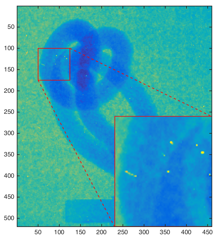
Example - Stripe removal in Fourier space
- Transform the image to Fourier space
- Multiply spectrum image by band pass filter
- Compute the inverse transform to obtain the filtered image in real space
plt.figure(figsize=[8,10])
plt.subplot(4,1,1);plt.imshow(plt.imread('ext-figures/lecture03/raw_img.png')); plt.title('$a$'); plt.axis('off');
plt.subplot(4,1,2);plt.imshow(plt.imread('ext-figures/lecture03/raw_spec.png')); plt.title('$\mathcal{F}(a)$'); plt.axis('off');
plt.subplot(4,1,3);plt.imshow(plt.imread('ext-figures/lecture03/filt_spec.png')); plt.title('Kernel $H$'); plt.axis('off');
plt.subplot(4,1,4);plt.imshow(plt.imread('ext-figures/lecture03/filt_img.png')); plt.title('$a_{filtered}$'); plt.axis('off');
The effect of the stripe filter
| Reconstructed CT slice before filter | Reconstructed CT slice after stripe filter |
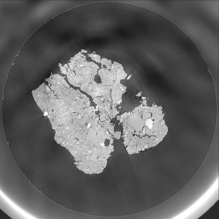 |
 |
Intensity variations are suppressed using the stripe filter on all projections.
Python functions
Filters in the spatial domain
e.g. from scipy import ndimage
ndimage.filters.convolve(f,h)Linear filter using kernel $h$ on image $f$.ndimage.filters.median_filter(f,\[n,m\])Median filter using an $n \times m$ filter neighborhood
Fourier transform
np.fft.fft2(f)Computes the 2D Fast Fourier Transform of image $f$np.fft.ifft2(F)Computes the inverse Fast Fourier Transform $F$.np.fft.fftshift()Rearranges the data to center the $\omega$=0. Works for 1D and 2D.
Complex numbers
np.abs(f), np.angle(f)Computes amplitude and argument of a complex number.np.real(f), np.imag(f)Gives the real and imaginary parts of a complex number.
Scale spaces
Why scale spaces?

Wavelets - the basic idea
- The wavelet transform produces scales by decomposing a signal into two signals at a coarser scale containing \emph{trend} and \emph{details}.\
- The next scale is computed using the trend of the previous transform
- The inverse transform brings $s$ back using $\{a_N,d_1, \ldots,d_N\}$.
- Many wavelet bases exists, the choice depends on the application.
Applications of wavelets
- Noise reduction
- Analysis
- Segmentation
- Compression

Wavelet transform of an image

Wavelet transform of an image - example
| Original | Wavelet transformed |
|---|---|
 |
 |
Wavelet noise reduction
The noise is found in the detail part of the WT
- Make a WT of the signal to a level that corresponds to the scale of the unwanted information.
- Threshold the detail part $d_{\gamma}=|d|<\gamma \,?\, 0 : d$.
- Inverse WT back to normal scale $\rightarrow$ image is filtered.


The starting point
The heat transport equation $$\frac{\partial T}{\partial t}=\kappa\,\nabla^2 T$$
- $T$ Image to filter (intensity $\equiv$ temperature)
- $\kappa$ Thermal conduction capacity
| Original | Iterations |
 |
Controlling the diffusivity
def g(x,lambd,n) :
    g=1/(1+(x/lambd)**n)
    return g
We want to control the diffusion process...
- Near edges The Diffusivity $\rightarrow$ 0
- Flat regions The Diffusivity $\rightarrow$ 1
The contrast function $G$ is our control function $$G(x)=\frac{1}{1+\left(\frac{x}{\lambda}\right)^n}$$
- $\lambda$ Threshold level
- $n$ Steepness of the threshold function
x=np.linspace(0,1,100);

plt.plot(x,g(x,lambd=0.5,n=12));
plt.xlabel('Image intensity (x)'); plt.ylabel('G(x)');plt.tight_layout()
Gradient controlled diffusivity
$$\frac{\partial u}{\partial t}=G(|\nabla u|)\,\nabla^2 u$$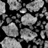 |
 |
| Image | Diffusivity map |
- $u$ Image to be filtered
- $G(\cdot)$ Non-linear function to control the diffusivity
- $\tau$ Time increment
- $N$ Number of iterations
The non-linear diffusion filter
A more robust filter is obtained with
$$\frac{\partial u}{\partial t}=G(|\nabla_{\sigma} u|)\,\nabla^2 u$$ - _$u$_ Image to be filtered - _$G(\cdot)$_ Non-linear function to control the contrast - _$\tau$_ Time increment per numerical iteration - _$N$_ Number of iterations - _$\nabla_{\sigma}$_ Gradient smoothed by a Gaussian filter, width $\sigma$Diffusion filter example
Neutron CT slice from a real-time experiment observing the coalescence of cold mixed bitumen.
| Original | Iterations of non-linear diffusion |
 |
Filtering as a regularization problem
The continued development
- 90's During the late 90's the diffusion filter was described in terms of a regularization problem.
- 00's Work toward regularization of total variation minimization.
TV-L1
$$u=\underset{u\in BV(\Omega)}{\operatorname{argmin}}\left\{\underbrace{|u|_{BV}}_{noise}+ \underbrace{\mbox{$\frac{\lambda}{2}$}\|f-u\|_{1}}_{fidelity}\right\}$$Rudin-Osher-Fatemi model (ROF)
$$u=\underset{u\in BV(\Omega)}{\operatorname{argmin}}\left\{\underbrace{|u|_{BV}}_{noise}+ \underbrace{\mbox{$\frac{\lambda}{2}$}\|f-u\|^2_{2}}_{fidelity}\right\}$$with $|u|_{BV}=\int_{\Omega}|\nabla u|^2$
The inverse scale space filter
The idea
We want smooth regions with sharp edges\ldots
- Turn the processing order of scale space filter upside down
- Start with an empty image
- Add large structures successively until an image with relevant features appears
The ISS filter - Some properties
- is an edge preserving filter for noise reduction.
- is defined by a partial differential equation.
- has a well defined termination point.
The ROF filter equation
The image $f$ is filtered by solving
$$\begin{eqnarray} \frac{\partial u}{\partial t}&=& \mathrm{div}\left(\frac{\nabla u}{|\nabla u|}\right)+\lambda\,(f-u+v)\nonumber\\ \frac{\partial v}{\partial t}&=& \alpha\, (f-u) \end{eqnarray}$$Variables:
- $f$ Input image
- $u$ Filtered image
- $v$ Regularization term (feedback of previous iteration)
Filter parameters
- $\lambda$ Related to the scale of the features to suppress.
- $\alpha$ Quality refinement
- $N$ Number of iterations
- $\tau$ Time increment


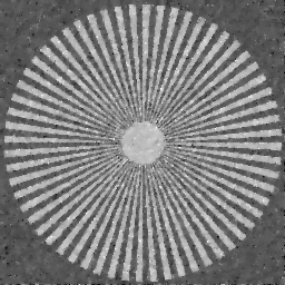

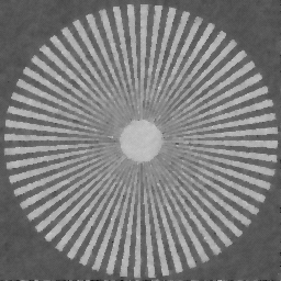
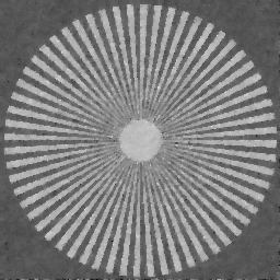


Non-local means
Non-local smoothing
The idea
Smoothing normally consider information from the neighborhood like
- Local averages (convolution)
- Gradients and Curvatures (PDE filters)
Non-local smoothing average similiar intensities in a global sense.
- Every filtered pixel is a weighted average of all pixels.
- Weights computed using difference between pixel intensities.
Filter definition
The non-local means filter is defined as $$u(p)=\frac{1}{C(p)}\sum_{q\in\Omega}v(q)\,f(p,q)$$ where
$v$ and $u$ input and result images.
$C(p)$ is the sum of all pixel weights as
$C(p)=\sum_{q\in\Omega}f(p,q)$
$f(p,q)$ is the weighting function
$f(p,q)=e^{-\frac{|B(q)-B(p)|^2}{h^2}}$
B(x) is a neighborhood operator e.g. local average around $x$
Performance complications
Problem
The orignal filter compares all pixels with all pixels\ldots\
- Complexity $\mathcal{O}(N^2)$
- Not feasible for large images, and particular 3D images!
Solution
It has been shown that not all pixels have to be compared to achieve a good filter effect. i.e. $\Omega$ in the filter equations can be replaced by $\Omega_i<<\Omega$
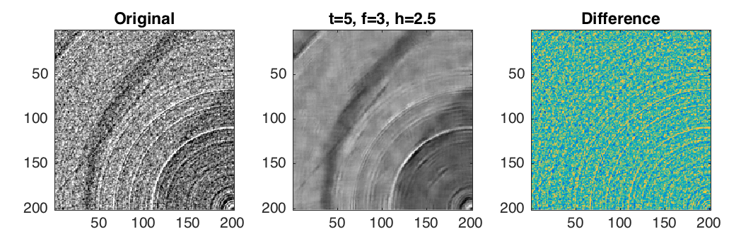
Verification using difference images
Compute pixel-wise difference between image $f$ and $g$

Difference images provide first diagnosis about processing performance
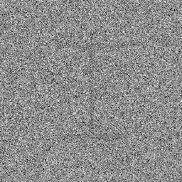
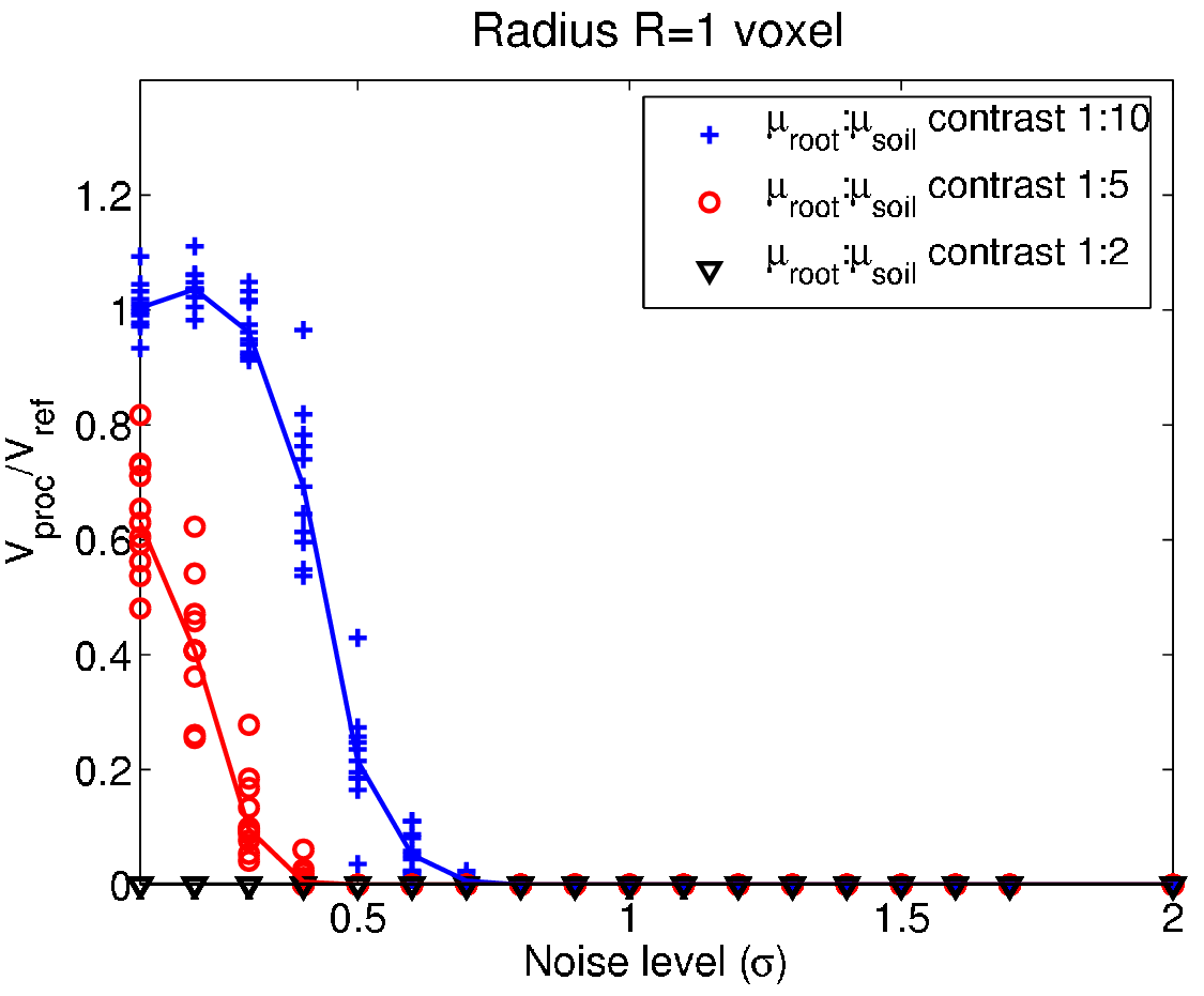
Performance testing - The smoke test
- Testing term from electronic hardware testing - drive the system until something fails due to overheating...
- In general: scan the parameter space for different SNR until the method fails to identify strength and weakness of the system.
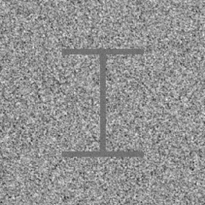
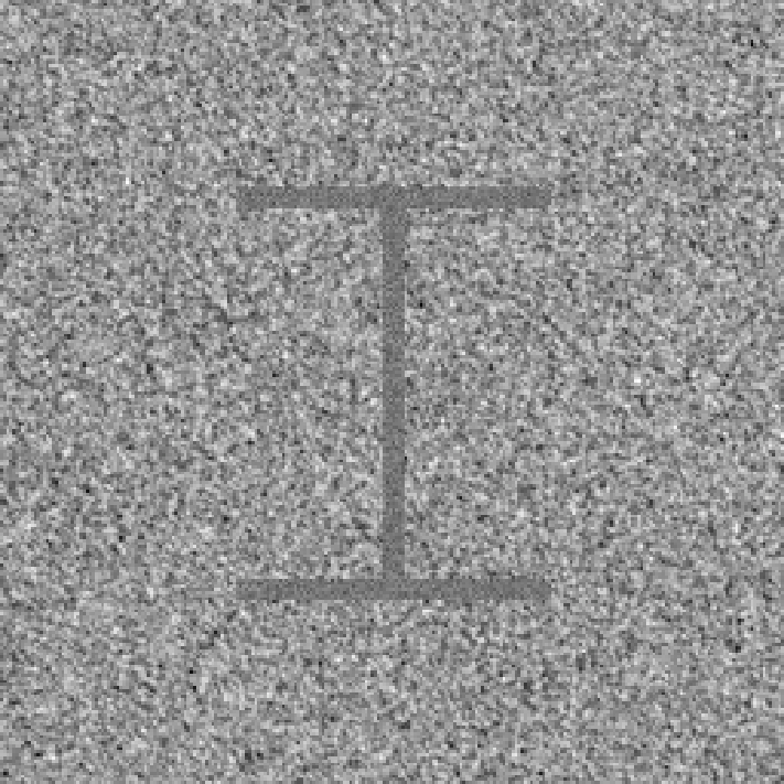
Test strategy
- Create a phantom image with relevant features.
- Add noise for different SNR to the phantom.
- Apply the processing method with different parameters.
- Measure the difference between processed and phantom.
- Repeat steps 2-4 $N$ times for better test statistics.
- Plot the results and identify the range of SNR and parameters that produce acceptable results.
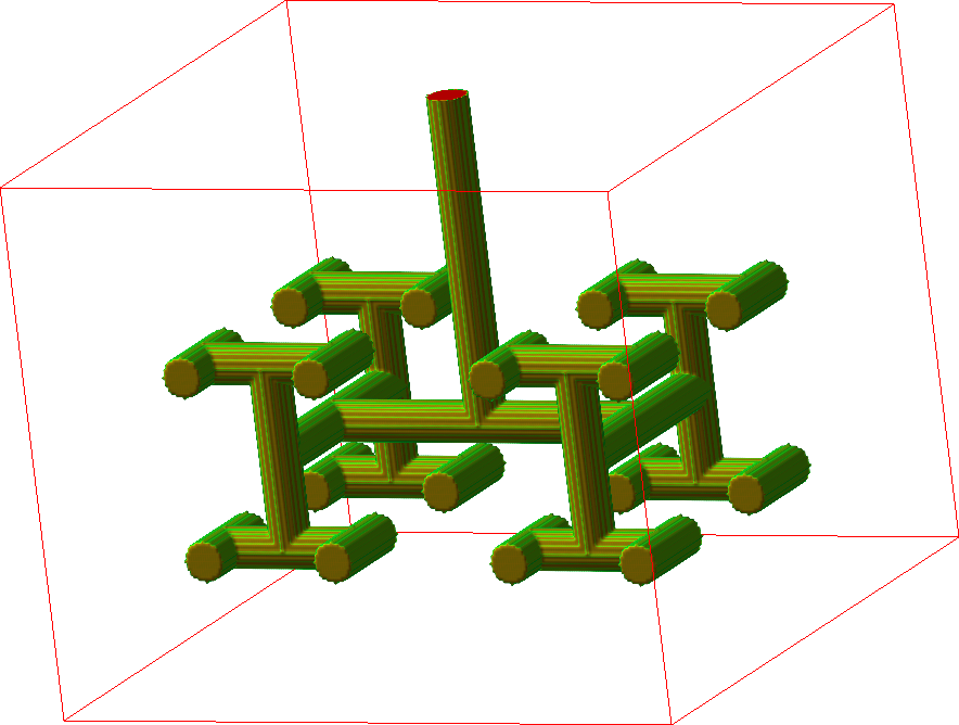
Data for evaluation - Phantom data
General purpose can be controlled
- Data with known features.
- Parameters can be changed.
- Shape
- Sharpness
- Contrast
- Noise (distribution and strength)

| 
|
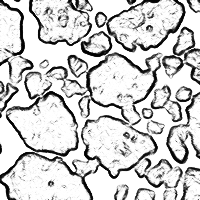
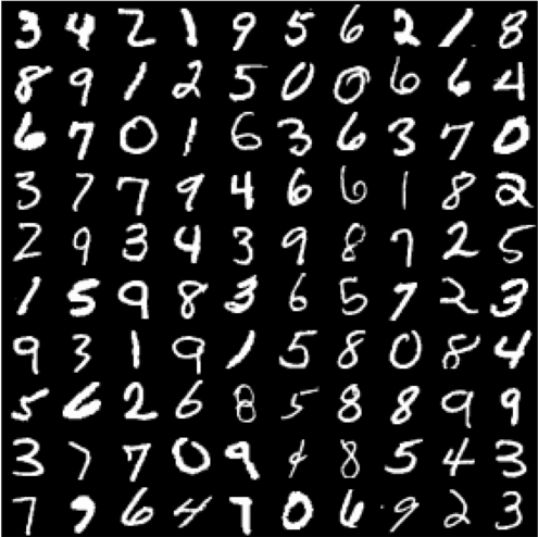
Data for evaluation - Labelled data
Often 'real' data
- Labeled by experts
- Used for training and validation
- Training of model
- Validation
- Test
Evaluation metrics for images
An evaluation procedure need a metric to compare the performance
Mean squared error
$$MSE(f,g)=\sum_{p\in \Omega}(f(p)-g(p))^2$$Structural similarity index
$$SSIM(f,g)=\frac{(2\mu_f\,\mu_g+C_1)(2\sigma_{fg}+C_2)}{(\mu_f^2+\mu_g^2+C_1)(\sigma_f^2+\sigma_g^2+C_2)}$$- $\mu_f$, $\mu_g$ Local mean of $f$ and $g$.
- $\sigma{fg}$_ Local correlation between $f$ and $g$.
- $\sigma_f$, $\sigma_g$ Local standard deviation of $f$ and $g$.
- $C_1$, $C_2$ Constants based on the image dynamics (small numbers).


Overview
Many filters

Details of filter performance

Take-home message
We have looked at different ways to suppress noise and artifacts:
- Convolution
- Median filters
- Wavelet denoising
- PDE filters
Which one you select depends on
- Purpose of the data
- Quality requirements
- Available time