Geospatial Data Science Applications: GEOG 4/590

Feb 21, 2022

Lecture 8: Visualization

Johnny Ryan: jryan4@uoregon.edu

Content of this lecture

• Plotting with matplotlib

* Mapping with `cartopy`

* Interactive plotting with `folium`

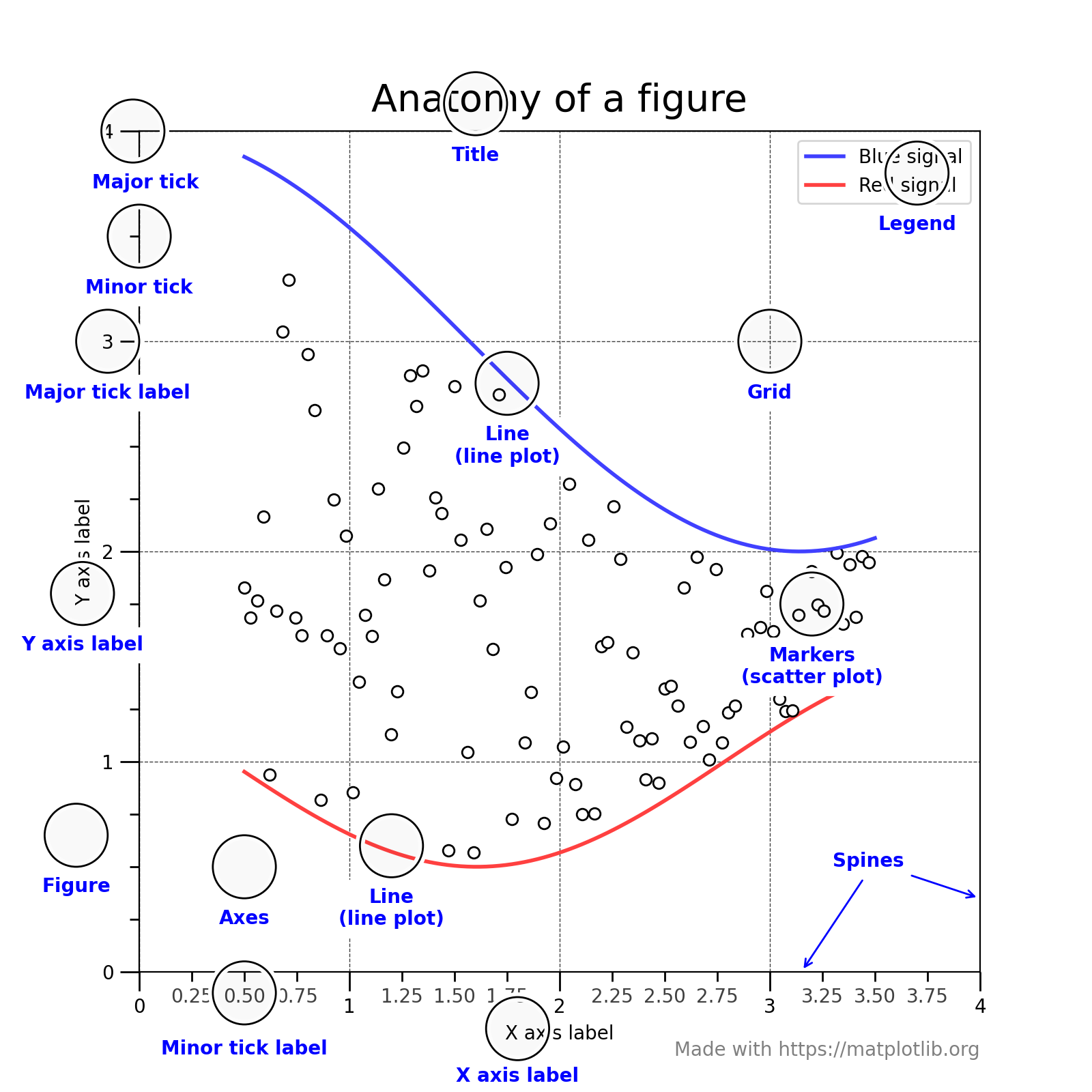
matplotlib

• The standard library for producing visualizations in Python

• Extremely comprehensive functionality

• Many different plot types and options to customize

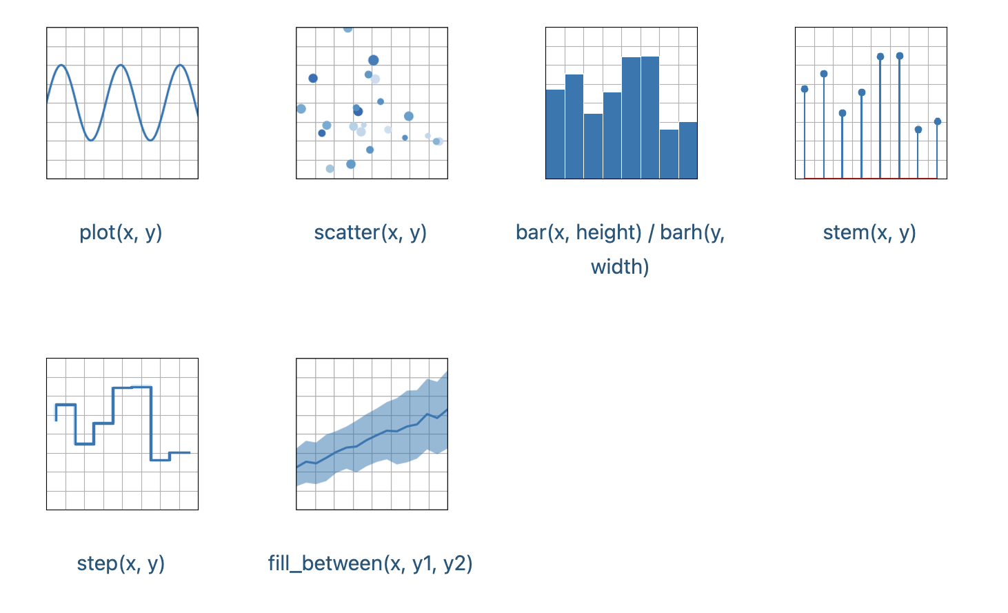
Basic

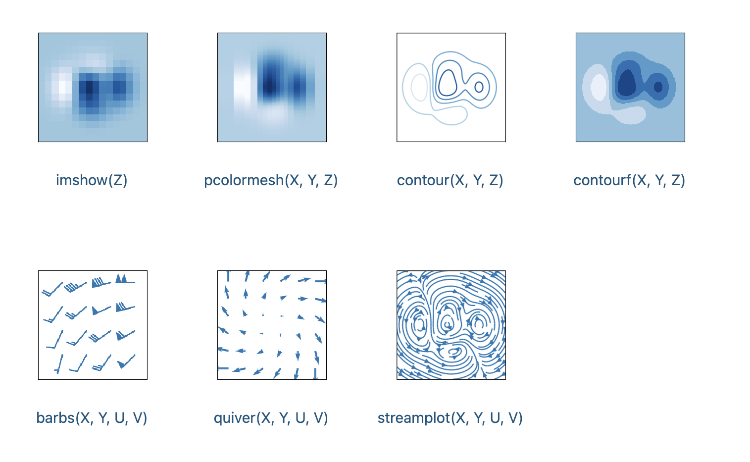
Arrays and fields

Statistics

# Import packages
import matplotlib.pyplot as plt
import numpy as np

Coding styles

There are essentially two ways to use matplotlib:

• 1. Explicitly create Figures and Axes, and call methods on them (the "object-oriented (OO) style")
• 2. Rely on pyplot to automatically create and manage the Figures and Axes and use pyplot functions for plotting

Pyplot style can be very convenient for quick interactive work

We recommend using the OO style for complicated plots that are intended to be reused as part of a larger project

Simple plot in matplotlib using "object-oriented (OO) style"

# Make data
x = np.linspace(0, 10, 100)
y = 4 + 2 * np.sin(2 * x)

# Create a figure containing a single axes
fig, ax = plt.subplots(figsize=(5,3)) # Set the figure size in inches 

# Plot data
ax.plot(x, y, linewidth=2.0) # Set linewidth in pixels
plt.show()

Simple plot in matplotlib using "pyplot style"

# Make data
x = np.linspace(0, 10, 100)
y = 4 + 2 * np.sin(2 * x)

# Plot data
plt.figure(figsize=(5, 3))
plt.plot(x, y, linewidth=2.0) # Set linewidth in pixels
plt.show()

Colors and line styles

# Create a figure containing a single axes
fig, ax = plt.subplots(figsize=(5,3)) # Set the figure size in inches 

# Plot data
ax.plot(x, y, linewidth=3.0, color='darkblue')
ax.plot(x, y+3, linewidth=2.0, color='red', linestyle='--')
plt.show()

Axes labels and legends

# Create a figure containing a single axes
fig, ax = plt.subplots(figsize=(5,3)) # Set the figure size in inches 

# Plot data
ax.plot(x, y, linewidth=3.0, color='darkblue', label='data1')
ax.plot(x, y+3, linewidth=2.0, color='red', linestyle='--', label='data2')

# Plot legend
ax.legend(fontsize=14)

# Set axes labels
ax.set_xlabel('Distance (km)', fontsize=14)
ax.set_ylabel('Elevation (m)', fontsize=14)

plt.show()

# Create a figure containing a single axes
fig, ax = plt.subplots(figsize=(5,3)) # Set the figure size in inches 

# Plot data
ax.plot(x, y, linewidth=3.0, color='darkblue', label='data1')
ax.plot(x, y+3, linewidth=2.0, color='red', linestyle='--', label='data2')

# Plot legend
ax.legend(fontsize=14)

# Set axes labels
ax.set_xlabel('Distance (km)', fontsize=14)
ax.set_ylabel('Elevation (m)', fontsize=14)

# Set grid style
ax.grid(linestyle='--', linewidth=1.5)

plt.show()

# Create a figure containing a single axes
fig, ax = plt.subplots(figsize=(5,3)) # Set the figure size in inches 

# Plot data
ax.plot(x, y, linewidth=3.0, color='darkblue', label='data1')

ax.set_xlabel('Distance (km)', fontsize=14) # Set axes labels
ax.set_ylabel('Elevation (m)', fontsize=14) # Set axes labels
ax.set_ylim(2, 6)                           # Set axes scale
ax.set_xticks(np.arange(0, 21, 1))          # Set tick labels
ax.yaxis.set_tick_params(labelsize=18)      # Set tick label size
ax.grid(False)                              # Hide grid lines
plt.show()

Produce a figure with two axes

# Create a figure containing two axes
fig, (ax1, ax2) = plt.subplots(ncols=2, nrows=1, figsize=(10,3)) 

# Plot data
ax1.plot(x, y, linewidth=2.0)
ax2.plot(x, y, linewidth=2.0)

plt.show()

Constrained layout

• Automatically adjusts subplots, legends and colorbars etc. so that they fit in the figure window while still preserving, as best they can, the logical layout requested by the user.

# Create a figure containing two axes
fig, (ax1, ax2) = plt.subplots(ncols=2, nrows=1, figsize=(10,3),
                               layout='constrained', sharey=True) 

# Plot data
ax1.plot(x, y, linewidth=2.0)
ax2.plot(x, y, linewidth=2.0)

plt.show()

More information

https://matplotlib.org/stable/tutorials/index.html

cartopy

• Package designed for geospatial data processing in order to produce maps and other geospatial data analyses

• Built using the powerful PROJ, numpy and shapely libraries and includes a programmatic interface built on top of matplotlib for the creation of publication quality maps.

# Import packages
import cartopy.crs as ccrs
import matplotlib.pyplot as plt

Simple map of world coastlines

# Create figure with no axes
fig = plt.figure(figsize=(10, 10))

# Define a GeoAxes instance with PlateCarree projection
ax = plt.axes(projection=ccrs.PlateCarree())

# Add coastlines to axes
ax.coastlines()
plt.show()

Add point data to map

# Coordinates of Seattle and London
seattle_lon, seattle_lat, london_lon, london_lat = -122, 47, 0, 52

fig = plt.figure(figsize=(10, 10)) # Create figure with no axes
ax = plt.axes(projection=ccrs.PlateCarree())
ax.set_extent([-130, 10, 30, 60], ccrs.Geodetic()) # Set extent

# Plot data
plt.plot([seattle_lon, london_lon], [seattle_lat, london_lat], color='red', 
         linewidth=2, transform=ccrs.Geodetic())

plt.plot([seattle_lon, london_lon], [seattle_lat, london_lat], color='blue', 
         linewidth=2, transform=ccrs.PlateCarree())

# Add coastlines to axes
ax.coastlines()

<cartopy.mpl.feature_artist.FeatureArtist at 0x1adb662f0>

Add gridded data to map

# Import packages
import xarray as xr

# Define filepath
filepath = '/Users/jryan4/Dropbox (University of Oregon)/Teaching/geospatial-data-science/data/lecture8/'

# Read data
tp = xr.open_dataset(filepath + 'era_2020_tp.nc')

tp['tp'].mean()

<xarray.DataArray 'tp' ()>
array(0.00232061, dtype=float32)

xarray.DataArray

'tp'

• 0.002321

  array(0.00232061, dtype=float32)

• Coordinates: (0)
• Attributes: (0)

# Create figure with no axes
fig = plt.figure(figsize=(10, 10))

# Define a GeoAxes instance with PlateCarree projection
ax = plt.axes(projection=ccrs.PlateCarree())
ax.set_global()
ax.coastlines()

ax.contourf(tp['longitude'], tp['latitude'], np.mean(tp['tp'], axis=0), 
            cmap='Blues')
plt.show()

Change projection systems

# Create figure with no axes
fig = plt.figure(figsize=(8, 8))

# Define a GeoAxes instance with LambertConformal projection
ax = plt.axes(projection=ccrs.LambertConformal())
ax.set_global()
ax.coastlines()

ax.contourf(tp['longitude'], tp['latitude'], np.mean(tp['tp'], axis=0), 
            cmap='Blues')
plt.show()

Change projection and define data transform

data_crs = ccrs.PlateCarree() # Specify data coordinate system
fig = plt.figure(figsize=(8, 8)) # Create figure with no axes

# Define a GeoAxes instance with PlateCarree projection
ax = plt.axes(projection=ccrs.LambertConformal())
ax.set_global()
ax.coastlines()

ax.contourf(tp['longitude'], tp['latitude'], np.mean(tp['tp'], axis=0), 
            transform=data_crs, cmap='Blues')
plt.show()

Set map extent

# Create figure with no axes
fig = plt.figure(figsize=(8, 8))
ax = plt.axes(projection=ccrs.LambertConformal())
ax.set_global()
ax.coastlines()

# Set extent 
ax.set_extent([-120, -70, 25, 48], crs=ccrs.PlateCarree())

ax.contourf(tp['longitude'], tp['latitude'], np.mean(tp['tp'], axis=0), 
            transform=data_crs, cmap='Blues')
plt.show()

folium

• Sometimes interactive, web-based displays of geospatial data are more useful/powerful than static figures

• folium is a web mapping framework based on Leaflet that allows us to produce interactive maps

# Import package
import folium

Basics

# Open a map at specific loction and zoom
m = folium.Map(location=[45.5236, -122.6750], zoom_start=11)
m

Make this Notebook Trusted to load map: File -> Trust Notebook

Tiles

• The default tiles are OpenStreetMap, but others tiles (e.g. Stamen Terrain, Stamen Toner) are built in. Some of them require an API key.

m = folium.Map(location=[45.372, -121.6972], zoom_start=12, tiles="Stamen Terrain")
m

Make this Notebook Trusted to load map: File -> Trust Notebook

Adding markers with labels

m = folium.Map(location=[45.372, -121.6972], zoom_start=12, tiles="Stamen Terrain")
folium.Marker([45.3288, -121.6625], 
              popup="<i>Mt. Hood Meadows</i>").add_to(m)
folium.Marker([45.3311, -121.7113], 
              popup="<b>Timberline Lodge</b>", 
              icon=folium.Icon(color="red", icon="info-sign")).add_to(m)
m

Make this Notebook Trusted to load map: File -> Trust Notebook

Chloropleth maps

# Import packages
import geopandas as gpd
import regionmask

# Define filepath
filepath = '/Users/jryan4/Dropbox (University of Oregon)/Teaching/geospatial-data-science/data/lecture8/'

# Read shapefile
states = gpd.read_file(filepath + 'us_mainland_states.shp')
states.crs

<Geographic 2D CRS: EPSG:4269>
Name: NAD83
Axis Info [ellipsoidal]:
- Lat[north]: Geodetic latitude (degree)
- Lon[east]: Geodetic longitude (degree)
Area of Use:
- name: North America - onshore and offshore: Canada - Alberta; British Columbia; Manitoba; New Brunswick; Newfoundland and Labrador; Northwest Territories; Nova Scotia; Nunavut; Ontario; Prince Edward Island; Quebec; Saskatchewan; Yukon. Puerto Rico. United States (USA) - Alabama; Alaska; Arizona; Arkansas; California; Colorado; Connecticut; Delaware; Florida; Georgia; Hawaii; Idaho; Illinois; Indiana; Iowa; Kansas; Kentucky; Louisiana; Maine; Maryland; Massachusetts; Michigan; Minnesota; Mississippi; Missouri; Montana; Nebraska; Nevada; New Hampshire; New Jersey; New Mexico; New York; North Carolina; North Dakota; Ohio; Oklahoma; Oregon; Pennsylvania; Rhode Island; South Carolina; South Dakota; Tennessee; Texas; Utah; Vermont; Virginia; Washington; West Virginia; Wisconsin; Wyoming. US Virgin Islands. British Virgin Islands.
- bounds: (167.65, 14.92, -47.74, 86.46)
Datum: North American Datum 1983
- Ellipsoid: GRS 1980
- Prime Meridian: Greenwich

# Convert coordinate system
states_wgs84 = states.to_crs('EPSG:4326')
states_wgs84.crs

<Geographic 2D CRS: EPSG:4326>
Name: WGS 84
Axis Info [ellipsoidal]:
- Lat[north]: Geodetic latitude (degree)
- Lon[east]: Geodetic longitude (degree)
Area of Use:
- name: World.
- bounds: (-180.0, -90.0, 180.0, 90.0)
Datum: World Geodetic System 1984 ensemble
- Ellipsoid: WGS 84
- Prime Meridian: Greenwich

Plot

• geopandas provides a high-level interface to the matplotlib library for making maps

states_wgs84.plot()

<AxesSubplot:>

Plot simple chloropleth map

states_wgs84.plot(column='ALAND')

<AxesSubplot:>

Saving figures

The recommended way to save plots for use outside of Jupyter notebooks is to use matplotlib's plt.savefig()

# Create a figure containing a single axes
fig, ax = plt.subplots(figsize=(5,3)) # Set the figure size in inches 
ax.plot(x, y, linewidth=3.0, color='darkblue')
ax.plot(x, y+3, linewidth=2.0, color='red', linestyle='--')
fig.savefig(filepath + 'plot.png', dpi=300, pad_inches=0.05,
        facecolor='white')