Space Invasion, Space Invaders, and Climate Change Mitigation
Scott Jeen
Jesus College MCR, 3rd June 2021
0. Prerequisites
- Agree that runaway climate change is worth avoiding
- Willing to accept approximations/back-of-the-envelope calcs
- Able to look beyond my UK-centric lens
0. Outline
1. Space Invasion: the footprint of climate change mitigation
2. Space Invaders: learning to control complex systems optimally
3. An Emission-minimisation Game
1. Space Invasion
High Carb(on) Diet
High Carb(on) Diet

Our Energy Diet
💡 → 1kWh
🥤 → 0.6kWh
🛁 → 5kWh
🚗 → 10kWh
💁♀️ → 125kWh/day or 5kW → 🎛🎛
after MacKay (2008)
Your Allotment for Growing Energy
- UK population: 66.65 million
- UK land area: 242,495 km²
- Your allotment: 3600m² ~ half a football pitch
- Your life: ~2.5 W/m$^2$

after MacKay (2008)
Energy Space Requirements
Your life: ~2.5 W/m$^2$
| Technology | ~ Power Per Unit Land Area | Zero Operational Emissions |
|---|---|---|
| Wind | 2.7 W/m$^2$ | 💚 |
| Biomass | 1 W/m$^2$ | 🤥 |
| Solar | 6 W/m$^2$ | 💚 |
| Hydropower | 0.9 W/m$^2$ | 🤥 |
| Geothermal | 3 W/m$^2$ | 💚 |
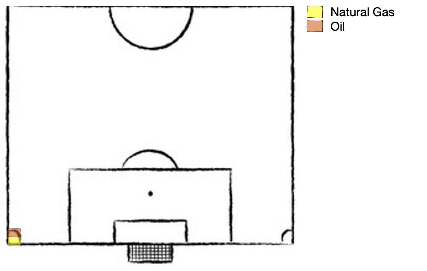
| Natural Gas | 1300 W/m$^2$ | ⛔️ |
| Coal | 125 W/m$^2$ | ⛔️ |
| Oil | 180 W/m$^2$ | ⛔️ |
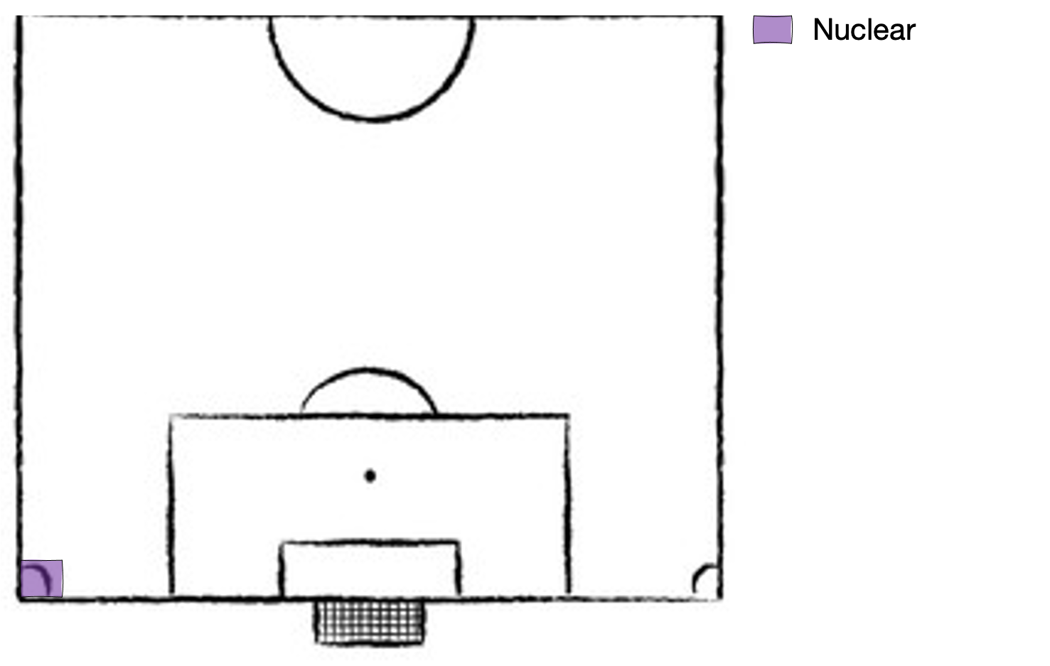
| Nuclear | 300 W/m$^2$ | 💚 |
Data: van Zalk & Behrens (2018)

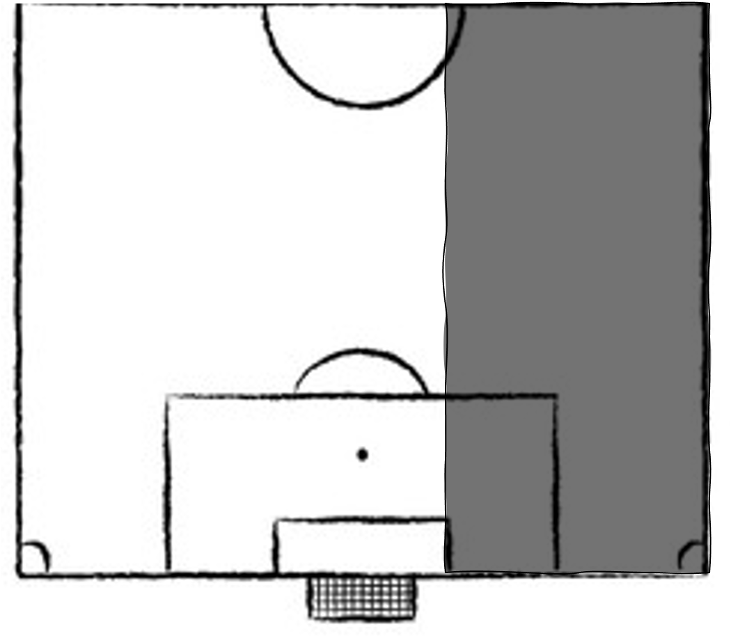
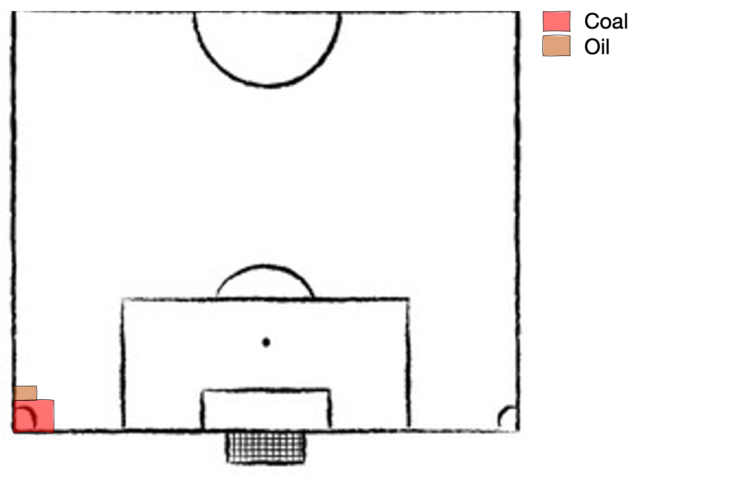
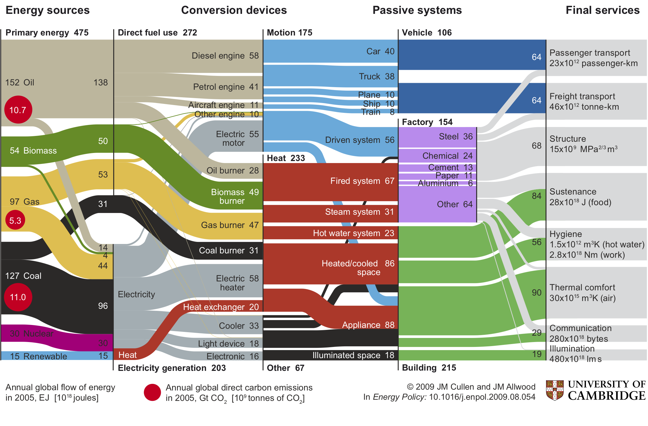
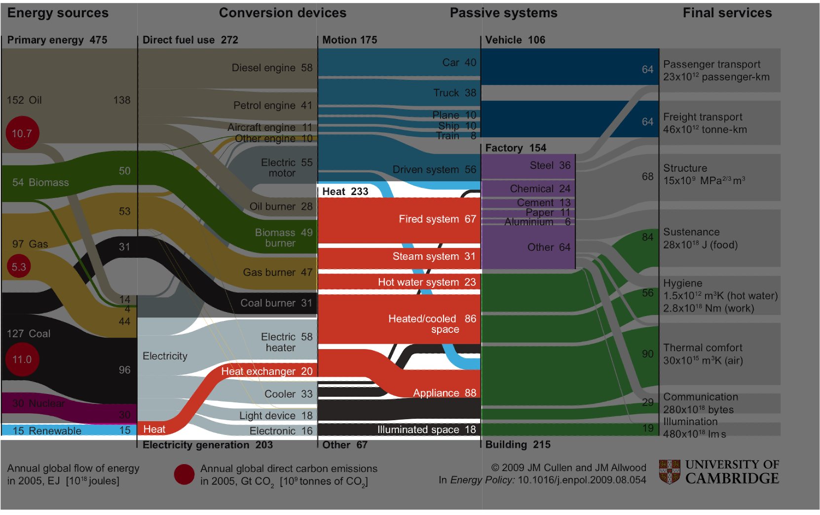
Then Mrs Thatcher came to power in the 1980s, closed most of the coal mines and replaced them with natural gas power plants of higher power densithy and lower emission intensity, and the energy mix looked something like this. Note: energy generation is using approximately 1% of land area here, plenty of room to continue live out the glorious 80s whilst the planet slowly begins to simmer.

If we were to generate energy using only wind and solar, we would use approximately 70% of UK land area, remember cities and countryside account for 40% of land area so we are eating into our leisure area now.

There are various ways to stop this space invasion, and one of them is to shrink the size of the energy pie; to use less energy in our society; to be more resource efficient. That is the focus of our research group's work, and that is one of the goals of my research. So, if we want to reduce our energy demand, what are our options, and where should our prioritises lie.
# animation function
def drawframe(n=int):
    x1 = x_new[:n]
    y1 = demand_new[:n]
    y2 = grid[:n]


    line1.set_data(x1, y1)
    line2.set_data(x1, y2)

    return (line1, line2)

# create animation
rc('animation', html='html5')
anim = animation.FuncAnimation(fig, drawframe, frames=len(x_new), interval=50)
# anim.save('images/intermittency.gif')
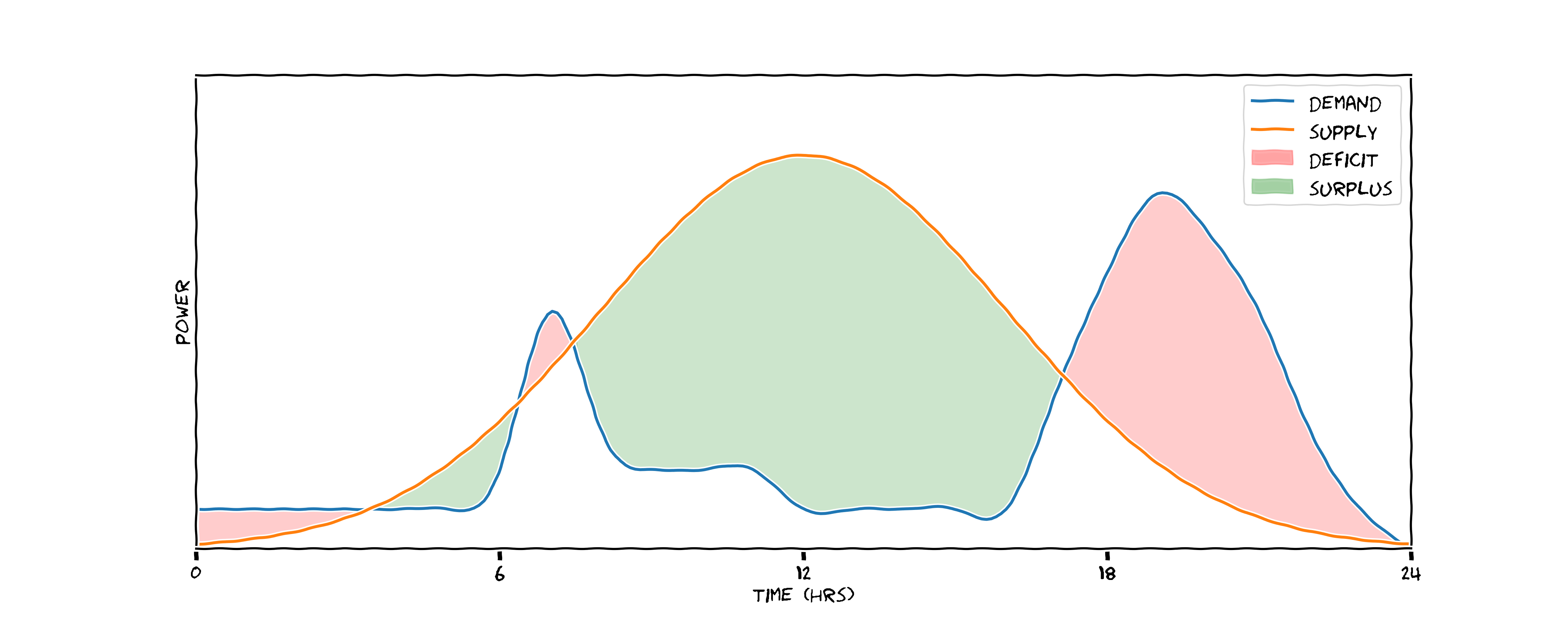
The Intermittency Problem
demand_new_2 = stats.norm.pdf(x_new, grid_mu, 6) * 80

# create fill between plot
with plt.xkcd():
    fig = plt.figure(figsize=(15,6))
    ax = plt.subplot(1,1,1)
    ax.set_xlabel('time (hrs)')
    ax.set_ylabel('power')
    plt.yticks([])
    plt.xticks([0,6,12,18,24])
    ax.set_xlim((0,24))
    ax.set_ylim((0,12))
    ax.plot(x_new, demand_new_2, label='demand')
    ax.plot(x_new, grid, label='supply')
    plt.fill_between(x_new, grid, demand_new_2, where=(demand_new_2>grid), color='blue', alpha=0.1, label='discharged')
    plt.fill_between(x_new, grid, demand_new_2, where=(demand_new_2<grid), color='orange', alpha=0.2,  label='stored')
    plt.legend()
    plt.savefig('images/opt_intermittency.png', dpi=300)

What we would prefer is a scenaario like this one. Here we've done two things: we flattened and broadened the demand curve, so there are no peaks to meet with natural gas; and we've introduced a storage medium - potentially a battery. During the hours of peak production we store energy (represented by orange) and we discharge this energy when needed, represented in blue. Here we've reduced our total energy demand by flattening the peak, and we've stopped the mitigated the problem of peak matching with natural gas - saving emissions in two ways.

Intermittency: A non-trivial optimsation problem
Stochastic supply:
- Weather-dependent
- Need accurate predictions of supply at varied time horizons: 5mins; 5 hours; 5 days
Stochastic demand:
- Depending on scenario, affected by countless variables
- Household setting: outdoor temperature; time of day; day of week
- Industrial setting: sales forecasts; raw material delivery schedules
2. Space Invaders
Reinforcement learning is the eminent paradigm for allowing computers to learn from experience. In RL, we consider an agent (represented by the brain) interacting with an environment (represented by the globe). The agent can take actions in an environment, and at each timestep step it receives feedback on how the state of the environment has changed given that action, and a reward for taking that action. The goal of the RL agent is to maximise the sum of cumulative rewards throughout its lifetime. When an RL agent is instantiated, it has no understanding of its environment or valuable actions to take in the environment, but learns by taking actions in the environment, in a trial and error fashion, observing the reward it accrues, and updating it's understanding of the state-space. It's hypothesised that this is much the same way we as humans learn intelligently. Consider the example of learning to ride a bike; we don't necessarily understand the physics of bike-riding, instead we get on the bike, try and balance and cycle and see what works for us. We find, through trial and error, the optimal way to position our body to balance the bike.
Although this appears a simple paradigm, it elicits extremelely powerful behaviour from computers.

from IPython.display import YouTubeVideo

YouTubeVideo('TmPfTpjtdgg', height=400, width=800)
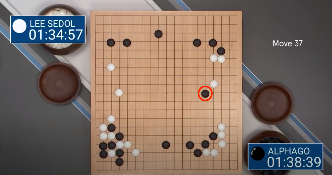
Here's another example, a few years later DeepMind created a Go-playing agent and played the world no.1 Lee Sedol in a 5 match series in South Korea. Go is considerably more complex game than chess; instead of an 8x8 board you have a 19x19 board, meaning the number of state permutations is astronimical. You can arrange the Go board in roughly $10^(170)$ permutations which is more atoms that are in the observable universe, meaning if you were to store each state permutation in a computer you would need one larger than the size of our universe.
AlphaGo beat Lee Sedol 4-1 having trained on a few millions episodes of game play, but perhaps the most intersting aspect of their match was the now infamous move 37 played by AlphaGo. On top is the board arrangement at move 37, apparently the most humans believe that with this board set-up the optimal stragey is the play in the margins, and avoid moving too close to the centre. AlphaGo elected to play 5 columns in from the margin, which flummoxed Lee Sedol and the audience of spectators, so much so that he had to go outside for a cigarette.
As the game evolved this move proved to be crucial. The board evolved in such that this black piece won AlphaGo the game, it from the near-infinite trajectories this game could have gone down, AlphaGo had correctly predicted the most likely. Not only did AlphaGo win the game, but it taught humans something about a complex system that we hadn't appreciated in the 3000 years we've been playing the game of Go, and to me that's really exciting.

To give you a little more intuition about what is happening under the hood of an RL agent, let's return quickly to the breakout example.
There are various ways in which the agent can represent its understanding of the system, but one is by assinging each part of the state-space (the environment) a value, and iterating it's formulation of that value as it receives rewards from the environment.
Here we see a plot of the agent's value estimate for the current state of the environment over time. We see a spikey pattern in the value estimate; just before the ball hits it bricks it has learned that it will receive reward shortly and estimates high value, then the value estimate drops as it knows it would receive more reward until some time into the future.
YouTubeVideo('DG17IKcDt8c', height=400, width=800)
3. An Emission-Minimising Game
So I've introduced RL, and discussed how agents can learn to play extremely complex games with no prior knowledge to a superhuman level. I've also motivated the need to reduce energy-use as a climate change mitigation technique. I'm going to conclude by combining these two sections together, and discuss formulating an emission-minimising game and how we can go about formulating a solution.
3.1 Formulating the Game
- Moves:
- Chiller control
- $\sum_{n=1}^6 a_t^n \in \mathcal{A}$, with $\mathcal{A} = [0\text{kW}, 5\text{kW}]$
- Goal:
- Minimise energy-use
- $\min{E_t}$, whilst
- Maintain temperature
- $T_t \leq 3^0C$
- Environment Dynamics:
- ?
Learning the Game Dynamics

3.2 Playing the Game
3.3. Winning the Game


3.4 Next Steps
- Incorportating grid randomness
- Incorporating uncertainty
- Online, data-efficient learning
- Multi-agent systems
Thanks!
References
Bossard, M., Feranec, J., & Otahel, J. (2000). CORINE land cover technical guide: Addendum 2000.
Cullen, J. M., & Allwood, J. M. (2010). The efficient use of energy: Tracing the global flow of energy from fuel to service. Energy Policy, 38(1), 75-81.
MacKay, D. (2008). Sustainable Energy-without the hot air. UIT cambridge.
Mnih, V., Kavukcuoglu, K., Silver, D., Graves, A., Antonoglou, I., Wierstra, D., & Riedmiller, M. (2013). Playing atari with deep reinforcement learning. arXiv preprint arXiv:1312.5602.
Silver, D., Schrittwieser, J., Simonyan, K., Antonoglou, I., Huang, A., Guez, A., ... & Hassabis, D. (2017). Mastering the game of go without human knowledge. nature, 550(7676), 354-359.
Silver, D. (2015). Lecture 1: Introduction to reinforcement learning. Google DeepMind, 1, 1-10.
van Zalk, J., & Behrens, P. (2018). The spatial extent of renewable and non-renewable power generation: A review and meta-analysis of power densities and their application in the US. Energy Policy, 123, 83-91.