CS236781: Deep Learning
Tutorial 3: Convolutional Neural Networks
Introduction
In this tutorial, we will cover:
- Convolutional layers
- Pooling layers
- Network architecture
- Spatial classification with fully-convolutional nets
- Residual nets
# Setup
%matplotlib inline
import os
import sys
import torch
import torchvision
import matplotlib.pyplot as plt
plt.rcParams['font.size'] = 20
data_dir = os.path.expanduser('~/.pytorch-datasets')
Theory Reminders
Multilayer Perceptron (MLP)
Model

Composed of multiple layers.
Each layer $j$ consists of $n_j$ regular perceptrons ("neurons") which calculate: $$ \vec{y}_j = \varphi\left( \mat{W}_j \vec{y}_{j-1} + \vec{b}_j \right),~ \mat{W}_j\in\set{R}^{n_{j}\times n_{j-1}},~ \vec{b}_j\in\set{R}^{n_j}. $$
- Note that both input and output are vectors. We can think of the above equation as describing a layer of multiple perceptrons.
- We'll henceforth refer to such layers as fully-connected or FC layers.
Given an input sample $\vec{x}^i$, the computed function of an $L$-layer MLP is: $$ \vec{y}_L^i= \varphi \left( \mat{W}_L \varphi \left( \cdots \varphi \left( \mat{W}_1 \vec{x}^i + \vec{b}_1 \right) \cdots \right)
- \vec{b}_L \right)
$$
Potent hypothesis class: An MLP with $L>1$, can approximate virtually any continuous function given enough parameters (Cybenko, 1989).
Limitations of MLPs for image classification
Number of parameters increases quadratically with image size due to connectivity.
- 28x28 MNIST image: 784 weights per neuron in the first layer
- 1000x1000x3 color image: 3M weights per neuron
Not enough compute
Overfitting
Fully-connected layers are highly sensitivity to translation, while image features are inherently translation-invariant.
Despite all these limitations we still want to use deep neural nets because they allow us to learn hierarchical, non-linear transformations of the input.
Convolutional Layers
We'll explain how convolutional layers work in using three different "views", from the most non-formal to the most formal.
Structural view
Just for intuition, a convolutional layer can be viewed as a composition of neurons (as in an FC layer) but with three important distinctions.
The neurons can be thought of as stacked in a 3D grid (insead of 1D).
Neurons that are at the same depth in the grid share the same weights (parameters $\mat{W},~\vec{b}$) (represented by color).
Each neuron is only connected to a small region of the previous layer's output (represented by location).
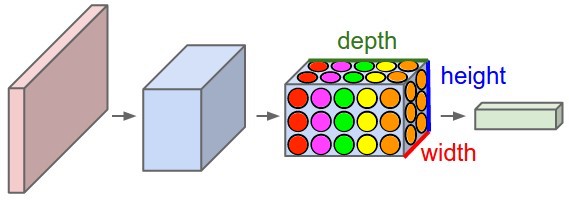
Crucially, each neuron is spatially local, but operates on the full depth dimension of its input layer.

Filter-based view
Since each neuron in a given depth-slice of operates on a small region of the input layer, we can think of the combined output of that depth-slice as a filtered version of the input volume.

Imagine sliding the filter along the input and computing an inner product at each point.

Since we have multiple depth-slices per convolutional layer, the layer computes multiple convolutions of the same input with different kernels (filters).
Each 2D slice of an input and output volume is known as feature map or a channel.
Formal definitions
Given an input tensor $\vec{x}$ of shape $(C_{\text{in}}, H_{\text{in}}, W_{\text{in}})$, a convolutional layer produces an output tensor $\vec{y}$ of shape $(C_{\text{out}}, H_{\text{out}}, W_{\text{out}})$, such that:
is the $j$-th feature map (or channel) of the output tensor $\vec{y}$, the $\ast$ denotes convolution, and $x^i$ is the $i$-th input feature map.
Recall the definition of the convolution operator: $$ \left\{\vec{g}\ast\vec{f}\right\}_j = \sum_{i} g_{j-i} f_{i}. $$

Note that in practice, correlation is used instead of convolution, as there's no need to "flip" a learned filter.
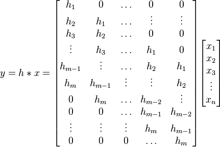
Convolution is a linear and shift-equivariant operator.
Linear means it can be represented simply as a matrix multiplication.
Shift-equivariance means that a shifted input will result in an output shifted by the same amount. Due to this property, the matrix representing a convolution is always a Toeplitz matrix.
Hyperparameters & dimentions
Assume an input volume of shape $(C_{\mathrm{in}}, H_{\mathrm{in}}, W_{\mathrm{in}})$, i.e. channels, height, width. Define,
- Number of kernels, $K \geq 1$.
- Spatial extent (size) of each kernel, $F \geq 1$.
- Stride $S\geq 1$: spatial distance between consecutive applications of a kernel.
- Padding $P\geq 0$: Number of "pixels" to zero-pad around each input feature map.
- Dilation $D \geq 1$: Spacing between kernel elements when applying to input.
In the following animations, blue maps are inputs, green maps are outputs and the shaded area is the kernel with $F=3$.
| $P=0,~S=1,~D=1$ | $P=1,~S=1,~D=1$ | $P=1,~S=2,~D=1$ | $P=0,~S=1,~D=2$ |
|---|---|---|---|
 |
 |
 |
 |
We can see that the second combination, $F=3,~P=1,~S=1,~D=1$, leads to identical sizes of input and output feature maps.
A 3D view
| $P=0,~S=1,~D=1$ | $P=1,~S=1,~D=1$ | $P=1,~S=2,~D=1$ |
|---|---|---|
 |
 |
 |
Then, given a set of hyperparameters,
Each convolution kernel will (usually) be a tensor of shape $(C_{\mathrm{in}}, F, F)$.
The ouput volume dimensions will be:
$$\begin{align} H_{\mathrm{out}} &= \left\lfloor \frac{H_{\mathrm{in}} + 2P - D\cdot(F-1) -1}{S} \right\rfloor + 1\\ W_{\mathrm{out}} &= \left\lfloor \frac{W_{\mathrm{in}} + 2P - D\cdot(F-1) -1}{S} \right\rfloor + 1\\ C_{\mathrm{out}} &= K\\ \end{align}$$
- The number of parameters in a convolutional layer will be:
Example: Input image is 1000x1000x3, and the first conv layer has $10$ kernels of size 5x5. The number of parameters in the first layer will be: $ 10 \cdot 3 \cdot 5^2 + 10 = 760 $.
Pytorch Conv2d layer example
import torchvision.transforms as tvtf

tf = tvtf.Compose([tvtf.ToTensor()])
ds_cifar10 = torchvision.datasets.CIFAR10(data_dir, download=True, train=True, transform=tf)
Files already downloaded and verified
# Load first CIFAR10 image
x0,y0 = ds_cifar10[0]

# add batch dimension
x0 = x0.unsqueeze(0)

# Note: channels come before spatial extent
print('x0 shape with batch dim:', x0.shape)
x0 shape with batch dim: torch.Size([1, 3, 32, 32])
# A function to count the number of parameters in an nn.Module.
def num_params(layer):
    return sum([p.numel() for p in layer.parameters()])
Let's create our first conv layer with pytorch:
import torch.nn as nn

# First conv layer: works on input image volume
conv1 = nn.Conv2d(in_channels=x0.shape[1], out_channels=10, padding=1, kernel_size=5, stride=1,dialation=1)

print(f'conv1: {num_params(conv1)} parameters')
conv1: 760 parameters
Number of parameters: $10\cdot(3\cdot3^2+1)=280$
# Apply the layer to an input
print(f'{"Input image shape:":25s}{x0.shape}')

y1 = conv1(x0)
print(f'{"After first conv layer:":25s}{y1.shape}')
Input image shape:       torch.Size([1, 3, 32, 32])
After first conv layer:  torch.Size([1, 10, 30, 30])
# Second conv layer: works on output volume of first layer
conv2 = nn.Conv2d(in_channels=10, out_channels=20, padding=0, kernel_size=7, stride=2)
print(f'conv2: {num_params(conv2)} parameters')

y2 = conv2(conv1(x0))
print(f'{"After second conv layer:":25s}{y2.shape}')
conv2: 9820 parameters
After second conv layer: torch.Size([1, 20, 12, 12])
New spatial extent:
$$ H_{\mathrm{out}} = \left\lfloor \frac{H_{\mathrm{in}} + 2P -F}{S} \right\rfloor + 1 = \left\lfloor \frac{32 + 2\cdot 0 -6}{2} \right\rfloor + 1 = 14 $$Note: observe that the width and height dimensions of the input image were never specified! more on the significance of that later.
Pooling layers
In addition to strides, another way to reduce the size of feature maps between the convolutional layers, is by adding pooling layers.
A pooling layer has the following hyperparameters (but no trainable parameters):
- Spatial extent (size) of each pooling kernel, $F \geq 2$.
- Stride $S\geq 2$: spatial distance between consecutive applications.
- Operation (e.g. max, average, $p$-norm)
Example: $\max$-pooling with $F=2,~S=2$ performing a factor-2 downsample:

Why pool feature maps after convolutions?
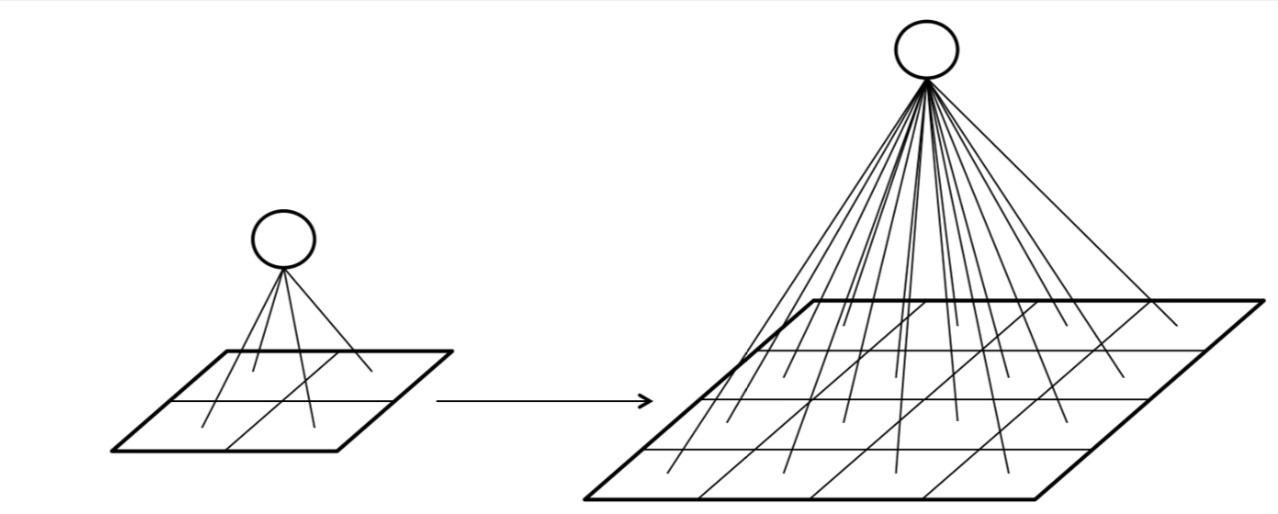
One reason is to more rapidly increase the receptive field of each layer.

- Receptive field size increases more rapidly if we add pooling, strides or dilation.
- We want successive conv layers to be affected by increasingly larger parts of the input image.
- This allows us to learn a hierarchy of visual features.

Another reason is to add invariance to changes in the input.
- Pooling within feature maps: introduces invariance to small translations
PyTorch Pool2d layer example
pool = nn.MaxPool2d(kernel_size=2, stride=2)

print(f'{"After second conv layer:":25s}{conv2(conv1(x0)).shape}')
print(f'{"After max-pool:":25s}{pool(conv2(conv1(x0))).shape}')
After second conv layer: torch.Size([1, 20, 12, 12])
After max-pool:          torch.Size([1, 20, 6, 6])
Network Architecture
The basic way to build an architecture of a deep convolutional neural net, is to repeat groups of conv-relu layers, optionally add pooling in between and end with an FC-softmax combination.
Why does such a scheme make sense, e.g. for image classification?

In the above image,
- all the conv blocks shown are actually conv-relu (or some other nonlinearity).
- The repeating conv-conv-...-pool blocks are learned, non-linear feature extractors: they learn to detect specific features in an image (e.g. lines at different orientations).
- The pooling controls the receptive field increase, so that more high-level features can be generated by each conv group (e.g. shapes composed from multiple simple lines).
- The FC-softmax at the end is just an MLP that uses the extracted features for classification.
- Training end-to-end learns the classifier together with the features!
- The rightmost architecture is called VGG, and used to be a relevant architecture for ImageNet classification.
- Other types of layers, such as normalization layers are usually also added.
There are many other things to consider as part of the architecture:
- Size of conv kernels
- Number of consecutive convolutions
- Use of batch normalization to speed up training
- Dropout for improved generalization
- Not using FC layers (we'll see later)
- Skip connections (we'll see later)
All of these could be hyperparameters to cross-validate over!
What filters are deep CNNs learning?
CNNs capture hierarchical features, with deeper layers capturing higher-level, class-specific features (Zeiler & Fergus, 2013).

PyTorch network architecture example
Let's implement LeNet, arguably the first successful CNN model for MNIST (LeCun, 1998).
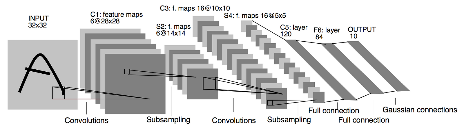
class LeNet(nn.Module):
    def __init__(self, in_channels=3):
        super().__init__()
        self.feature_extractor = nn.Sequential(
            nn.Conv2d(in_channels, out_channels=6, kernel_size=5),
            nn.ReLU(),
            nn.MaxPool2d(2),
            nn.Conv2d(in_channels=6, out_channels=16, kernel_size=5),
            nn.ReLU(),
            nn.MaxPool2d(2),
        )
        self.classifier = nn.Sequential(
            nn.Linear(16*5*5, 120),  # Why 16*5*5 ?
            nn.ReLU(),
            nn.Linear(120, 84), # (N, 120) -> (N, 84)
            nn.ReLU(),
            nn.Linear(84, 10)   # (N, 84)  -> (N, 10)
        )
    def forward(self, x):
        features = self.feature_extractor(x)
        features = features.view(features.size(0), -1)
        class_scores = self.classifier(features)
        return class_scores
net = LeNet()
print(net)
LeNet(
  (feature_extractor): Sequential(
    (0): Conv2d(3, 6, kernel_size=(5, 5), stride=(1, 1))
    (1): ReLU()
    (2): MaxPool2d(kernel_size=2, stride=2, padding=0, dilation=1, ceil_mode=False)
    (3): Conv2d(6, 16, kernel_size=(5, 5), stride=(1, 1))
    (4): ReLU()
    (5): MaxPool2d(kernel_size=2, stride=2, padding=0, dilation=1, ceil_mode=False)
  )
  (classifier): Sequential(
    (0): Linear(in_features=400, out_features=120, bias=True)
    (1): ReLU()
    (2): Linear(in_features=120, out_features=84, bias=True)
    (3): ReLU()
    (4): Linear(in_features=84, out_features=10, bias=True)
  )
)
# Test forward pass
print('x0 shape=', x0.shape, end='\n\n')
print('LeNet(x0)=', net(x0), end='\n\n')
print('shape=', net(x0).shape)
x0 shape= torch.Size([1, 3, 32, 32])

LeNet(x0)= tensor([[-0.0388,  0.0337, -0.0120, -0.0205, -0.0326,  0.0651, -0.0826, -0.0595,
          0.0831,  0.1228]], grad_fn=<AddmmBackward0>)

shape= torch.Size([1, 10])
Fully-convolutional Networks
you can read at home, not for the homework
Residual Networks

For image-related tasks it seems that deeper is better: learn more complex features.
How deep can we go? Should more depth always improve results?
In theory, adding an addition layer should provide at least the same accuracy as before.
Extra layers could always be just identity maps.
In practice, there are two major problems with adding depth:
- More difficult convergence: vanishing gradients
- More difficult optimization: parameter space increases

I.e., even if the same solution (or better) exists, SGD-based optimization can't find it. Optimization error increased with depth.
ResNets attempt to address these issues by building a network architecture composed of convolutional blocks with added shortcut-connections:

(Left: basic block; right: bottleneck block).
Here the weight layers are 3x3 or 1x1 convolutions followed by batch-normalization.
Why do these shortcut-connections help?
These shortcuts create two key advantages:
- Allow gradients to "flow" freely backwards
- Each block only learns the "residual mapping", i.e. some delta from the identity map which is easier to optimize.
Implementation: In the homeworks :)
Thanks!