Notebook

< Modules | CNN & LSTM | Transfer Learning >¶

Convolutional Neural Networks & Recurrent Neural Networks¶

sprinke deep learning

Google Colab only!¶

In [ ]:

# execute only if you're using Google Colab
!wget -q https://raw.githubusercontent.com/ahug/amld-pytorch-workshop/master/binder/requirements.txt -O requirements.txt
!pip install -qr requirements.txt

In [ ]:

%matplotlib inline

import numpy as np

import torch
import torch.nn as nn
import torch.nn.functional as F
import torch.optim as optim
from torchvision import datasets, transforms

import matplotlib.pyplot as plt

from collections import OrderedDict
import colorama

In [ ]:

import ipywidgets as widgets
from ipywidgets import interact, interactive, fixed, interact_manual

Let's define the LeNet-5 architecture¶

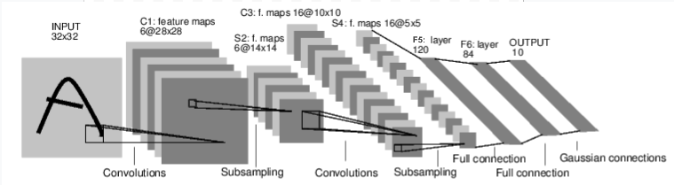
Y. LeCun, L. Bottou, Y. Bengio, and P. Haffner. "Gradient-based learning applied to document recognition." Proceedings of the IEEE, 86(11):2278-2324, November 1998.

Note: The Gaussian connections in the last layer are euclidean radial basis functions for each class to estimate the lack of fit. In our implementation, we use a cross-entropy loss function as it's common nowadays.

In [ ]:

class LeNet5(nn.Module):
    def __init__(self):
        super(LeNet5, self).__init__()
        
        self.conv_net = nn.Sequential(OrderedDict([
            ('C1', nn.Conv2d(1, 6, kernel_size=(5, 5))),
            ('Relu1', nn.ReLU()),
            
            ('S2', nn.MaxPool2d(kernel_size=(2, 2), stride=2)),
            ('C3', nn.Conv2d(6, 16, kernel_size=(5, 5))),
            ('Relu3', nn.ReLU()),
            
            ('S4', nn.MaxPool2d(kernel_size=(2, 2), stride=2)),
            ('C5', nn.Conv2d(16, 120, kernel_size=(5, 5))),
            ('Relu5', nn.ReLU()),
        ]))
        
        self.fully_connected = nn.Sequential(OrderedDict([
            ('F6', nn.Linear(120, 84)),
            ('Relu6', nn.ReLU()),
            ('F7', nn.Linear(84, 10)),
            ('LogSoftmax', nn.LogSoftmax(dim=-1))
        ]))
        
        
    def forward(self, imgs):
        output = self.conv_net(imgs)
        output = output.view(imgs.shape[0], -1)  # imgs.shape[0] == batch_size
        output = self.fully_connected(output)
        return output        

An extensive list of all available layer types can be found on https://pytorch.org/docs/stable/nn.html.

Print a network summary¶

In [ ]:

conv_net = LeNet5()
print(conv_net)

Retrieve trainable parameters¶

In [ ]:

named_params = list(conv_net.named_parameters())
print("len(params): %s\n" % len(named_params))
for name, param in named_params:
    print("%s:\t%s" % (name, param.shape))

Feed network with a random input¶

In [ ]:

input = torch.randn(1, 1, 32, 32)  # batch_size, num_channels, height, width
out = conv_net(input)
print("Log-Probabilities: \n%s\n" % out)
print("Probabilities: \n%s\n" % torch.exp(out))
print("out.shape: \n%s" % (out.shape,))

How can we now actually train our CNN?¶

In [ ]:

def train_cnn(model, train_loader, test_loader, device, num_epochs=3, lr=0.1, use_scheduler=False):
    model.train()  # not necessary in our example, but still good practice since modules
                   # like nn.Dropout, nn.BatchNorm require it
        
    # define an optimizer
    optimizer = torch.optim.Adam(model.parameters(), lr=lr)
    criterion = torch.nn.CrossEntropyLoss()
    
    if use_scheduler:
        scheduler = torch.optim.lr_scheduler.StepLR(optimizer, 1, 0.85)

    for epoch in range(num_epochs):
        print("="*40, "Starting epoch %d" % (epoch + 1), "="*40)
        
        model.train()  # reset to train mode after accuracy computation
        
        if use_scheduler:
            scheduler.step()
        
        # dataloader returns batches of images for 'data' and a tensor with their respective labels in 'labels'
        for batch_idx, (data, labels) in enumerate(train_loader):
            data, labels = data.to(device), labels.to(device)

            optimizer.zero_grad()
            
            output = model(data)
            loss = criterion(output, labels)
            loss.backward()
            optimizer.step()
            
            
            if batch_idx % 40 == 0:
                print("Batch %d/%d, Loss=%.4f" % (batch_idx, len(train_loader), loss.item()))

        train_acc = accuracy(model, train_loader, device)
        test_acc = accuracy(model, test_loader, device)
        print(colorama.Fore.GREEN, "\nAccuracy on training: %.2f%%" % (100*train_acc))
        print("Accuracy on test: %.2f%%" % (100*test_acc), colorama.Fore.RESET)

Evaluate model's accuracy on train/test data¶

In [ ]:

def accuracy(model, dataloader, device):
    """ Computes the model's accuracy on the data provided by 'dataloader'
    """
    model.eval()
    
    num_correct = 0
    num_samples = 0
    with torch.no_grad():  # deactivates autograd, reduces memory usage and speeds up computations
        for data, labels in dataloader:
            data, labels = data.to(device), labels.to(device)

            predictions = model(data).max(1)[1]  # indices of the maxima along the second dimension
            num_correct += (predictions == labels).sum().item()
            num_samples += predictions.shape[0]
        
    return num_correct / num_samples

How to load the training/test data: dataloaders¶

In [ ]:

train_data = datasets.MNIST('./data', 
                            train = True, 
                            download = True,
                            transform = transforms.Compose([
                                transforms.Resize((32, 32)),
                                transforms.ToTensor()
                            ]))

test_data = datasets.MNIST('./data', 
                            train = False, 
                            download = True,
                            transform = transforms.Compose([
                                transforms.Resize((32, 32)),
                                transforms.ToTensor()
                            ]))

train_loader = torch.utils.data.DataLoader(train_data, batch_size=256, shuffle=True)
test_loader = torch.utils.data.DataLoader(test_data, batch_size=1024, shuffle=True)

Let's visualize some of the training samples¶

In [ ]:

plt.figure(figsize=(16,9))
data, target = next(iter(train_loader))
for i in range(10):
    img = data.squeeze(1)[i]
    plt.subplot(1, 10, i+1)
    plt.imshow(img, cmap="gray", interpolation="none")
    plt.xlabel(target[i].item(), fontsize=18)
    plt.xticks([])
    plt.yticks([])    

Start the training!¶

In [ ]:

device = torch.device('cuda' if torch.cuda.is_available() else 'cpu')
conv_net = conv_net.to(device)

train_cnn(conv_net, train_loader, test_loader, device, lr=2e-3)

Let's look at some of the model's predictions¶

In [ ]:

def visualize_predictions(model, dataloader, device):
    data, labels = next(iter(dataloader))
    data, labels = data[:10].to(device), labels[:10]
    predictions = model(data).max(1)[1]
    
    predictions, data = predictions.cpu(), data.cpu()
    
    plt.figure(figsize=(16,9))
    for i in range(10):
        img = data.squeeze(1)[i]
        plt.subplot(1, 10, i+1)
        plt.imshow(img, cmap="gray", interpolation="none")
        plt.xlabel(predictions[i].item(), fontsize=18)
        plt.xticks([])
        plt.yticks([])    
    
visualize_predictions(conv_net, test_loader, device)

We might look at the LSTM example later if we still have some time left¶

Long-Short Term Memory (LSTM)¶

Long short-term memory (LSTM) are units of a recurrent neural network. They were proposed by Hochreiter et al. in 1997. The LSTM was designed to overcome the vanishing gradient problem which was inherent to most recurrent neural networks in these days. The vanishing gradient problem becomes especially problematic for longer sequences (such as text) where they significantly slow down learning or in the worst case even prevent convergence.

Note: They still don't solve the exploding gradient - a commonly used heuristic is to clip the gradients at a certain threshold.

Illustration by Christopher Olah: http://colah.github.io/posts/2015-08-Understanding-LSTMs/

How to use the torch.nn.LSTM module¶

We can setup a simple LSTM using the 'torch.nn.LSTM' class

In [ ]:

lstm = torch.nn.LSTM(input_size=10, hidden_size=20, num_layers=2)
dummy_input = torch.randn(5, 3, 10) # (seq_length, batch_size, num_features)
h0 = torch.randn(2, 3, 20)
c0 = torch.randn(2, 3, 20)
output, (hn, cn) = lstm(dummy_input, (h0, c0))

print("output.shape: \n%s\n" % (output.shape,))
print("hn.shape: \n%s\n" % (hn.shape,))
print("cn.shape: \n%s" % (cn.shape,))

output contains the hidden states of the last layer for all the timesteps. hn and cn contain only the hidden/cell state of the last timestep. Therefore, the last slice of output is actually identical to the hidden state of the last layer.

In [ ]:

print("output[-1,:,:]: \n%s\n" % output[-1, :, :])
print("hn[1:,:,:]: \n%s" % hn[1, :, :])

Toy Example - Image classification using an LSTM¶

We can again define our model by subclassing 'nn.Module':

In [ ]:

class ImageLSTM(nn.Module):
    def __init__(self, num_features, seq_length, hidden_size, num_layers, num_classes):
        super(ImageLSTM, self).__init__() 
        self.num_features = num_features
        self.seq_length = seq_length
        self.num_layers = num_layers
        self.hidden_size = hidden_size
        
        self.lstm = nn.LSTM(num_features, hidden_size, num_layers, batch_first=True) 
        # input.shape = (batch_size, seq_length, num_features)
        # if batch_first is 'False' (default) it requires the input to be of
        # shape = (seq_len, batch_size, num_features)
        self.linear = nn.Linear(hidden_size, num_classes)
        
        
    def forward(self, x):
        x = x.squeeze(1).permute(0, 2, 1).view(-1, self.seq_length, self.num_features)  # read from left-to-right
        
        # Set initial hidden and cell states
        h0 = torch.zeros(self.num_layers, x.size(0), self.hidden_size).to(x.device) 
        c0 = torch.zeros(self.num_layers, x.size(0), self.hidden_size).to(x.device)
        
        # Forward propagate LSTM
        out, _ = self.lstm(x, (h0, c0))  # out: tensor of shape (batch_size, seq_length, hidden_size)
                                         #      --> output of last layer
        
        # Decode the hidden state of the last time step
        out = self.linear(out[:, -1, :])
        return F.log_softmax(out, dim=1)

In [ ]:

lstm_model = ImageLSTM(num_features=32, seq_length=32, hidden_size=10, num_layers=3, num_classes=10)
lstm_model = lstm_model.to(device)

train_cnn(lstm_model, train_loader, test_loader, device, use_scheduler=True)

See the model in action!¶

We can look at the outputs of the model which gives us probability estimates for each class

In [ ]:

data, target = next(iter(train_loader))  # get a sample from the dataloader

output = lstm_model(data.to(device))
output = output.cpu()

plt.figure(figsize=(15,5))
plt.subplot(1, 2, 1)
plt.imshow(data[0, 0, :, :], cmap="gray", interpolation="None")
plt.subplot(1, 2, 2)
plt.title("Predicted probabilities")
plt.ylim([0, 1])
plt.bar(torch.arange(10), torch.exp(output[0]).data, tick_label=np.arange(10))

Our LSTM reads the image from left-to-right. So how does the prediction change while reading the image? Use the slider below to explore it yourself!

In [ ]:

img = data[0, 0, :, :].view(32, 32)

probs = []
for ix in range(1, 33):
    lstm_model.seq_length = ix
    input = img[:, :ix].view(1, 32, -1).contiguous()
    output = lstm_model(input.to(device)).view(-1)
    probs.append(torch.exp(output[target[0].item()]).item())

    
def draw(width):
    img = data[0, :, :, :].clone().view(32, 32) # get first image from batch
    plt.figure(figsize=(16,9))
    
    mask = torch.zeros(32, 32)
    mask[:, :width] = 1
    
    # draw image with mask
    plt.subplot(221)
    plt.imshow(img, cmap="gray", interpolation="none")
    plt.imshow(mask, cmap="gray", alpha=0.6, interpolation="none")

    plt.subplot(222)
    plt.title("$P(X=%d)$" % target[0])
    plt.ylim([0, 1])
    plt.plot(np.arange(1, 33), probs)
    plt.plot(width, probs[width-1], 'or')  
    
    
    lstm_input = img[:, :width].view(1, 32, -1).contiguous().to(device)
    lstm_model.seq_length = width
    output = lstm_model(lstm_input).cpu()
    plt.subplot(212)
    plt.title("Predicted probabilities")
    plt.ylim([0, 1])
    plt.bar(torch.arange(10), torch.exp(output[0]).data, tick_label=np.arange(10))
        

interactive_plot = interact(draw, width=widgets.IntSlider(min=1, max=31, step=1))
interactive_plot

Don't forget to download the notebook, otherwise your changes will be lost!¶

Download the notebook

< Modules | CNN & LSTM | Transfer Learning >¶