Molecular mechnism of earliest and fastest appearance of megakaryocytes
One intriguing phenomenon observed in hematopoiesis is that commitment to and appearance of the Meg lineage occurs more rapidly than other lineages (Sanjuan-Pla et al., 2013; Yamamoto et al., 2013). However, the mechanisms underlying this process remain elusive. To mechanistically dissect this finding, we focused on all cell types derived from the MEP-like lineage.
In this tutorial, we will guide you to
- learn vector field and manually select fixed points
- visualize topography with computed fixed points
- compute pseudotime (potential)
- visualize vector field pseudotime of cell types
Import relevant packages
%%capture
import numpy as np
import pandas as pd
import matplotlib.pyplot as plt
# import Scribe as sb
import sys
import os
# import scanpy as sc
import dynamo as dyn
import seaborn as sns
dyn.dynamo_logger.main_silence()
# filter warnings for cleaner tutorials
import warnings
warnings.filterwarnings('ignore')
adata_labeling = dyn.sample_data.hematopoiesis()
take a glance at what is in adata object. All observations, embedding layers and other data in adata are computed within dynamo. Please refer to other dynamo tutorials regarding how to obtain these values from metadata and raw new/total and (or) raw spliced/unspliced gene expression values.
A schematic of leveraging differential geometry
- ranking genes (using either raw or absolute values) across all cells or in each cell group/state
- gene set enrichment, network construction, and visualization
- identifying top toggle-switch pairs driving cell fate bifurcations

Visualize topography
Lineage tree of hematopoiesis, lumped automatically from the vector field built in the UMAP space
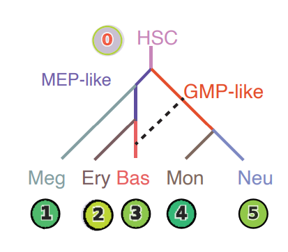
The reconstructed vector field and associated fixed points.
The color of digits in each node reflects the type of fixed point: red, emitting fixed point; black, absorbing fixed point. The color of the numbered nodes corresponds to the confidence of the fixed points.
Manually select good fixed points found by topography
adata_labeling.uns["VecFld_umap"].keys()
dict_keys(['C', 'E_traj', 'P', 'V', 'VFCIndex', 'X', 'X_ctrl', 'X_data', 'Xss', 'Y', 'beta', 'confidence', 'ctrl_idx', 'ftype', 'grid', 'grid_V', 'iteration', 'method', 'nullcline', 'sigma2', 'tecr_traj', 'valid_ind', 'xlim', 'ylim'])
dyn.vf.topography(adata_labeling, n=750, basis="umap")
AnnData object with n_obs × n_vars = 1947 × 1956
obs: 'batch', 'time', 'cell_type', 'nGenes', 'nCounts', 'pMito', 'pass_basic_filter', 'new_Size_Factor', 'initial_new_cell_size', 'total_Size_Factor', 'initial_total_cell_size', 'spliced_Size_Factor', 'initial_spliced_cell_size', 'unspliced_Size_Factor', 'initial_unspliced_cell_size', 'Size_Factor', 'initial_cell_size', 'ntr', 'cell_cycle_phase', 'leiden', 'control_point_pca', 'inlier_prob_pca', 'obs_vf_angle_pca', 'pca_ddhodge_div', 'pca_ddhodge_potential', 'acceleration_pca', 'curvature_pca', 'n_counts', 'mt_frac', 'jacobian_det_pca', 'manual_selection', 'divergence_pca', 'curv_leiden', 'curv_louvain', 'SPI1->GATA1_jacobian', 'jacobian', 'umap_ori_leiden', 'umap_ori_louvain', 'umap_ddhodge_div', 'umap_ddhodge_potential', 'curl_umap', 'divergence_umap', 'acceleration_umap', 'control_point_umap_ori', 'inlier_prob_umap_ori', 'obs_vf_angle_umap_ori', 'curvature_umap_ori'
var: 'gene_name', 'gene_id', 'nCells', 'nCounts', 'pass_basic_filter', 'use_for_pca', 'frac', 'ntr', 'time_3_alpha', 'time_3_beta', 'time_3_gamma', 'time_3_half_life', 'time_3_alpha_b', 'time_3_alpha_r2', 'time_3_gamma_b', 'time_3_gamma_r2', 'time_3_gamma_logLL', 'time_3_delta_b', 'time_3_delta_r2', 'time_3_bs', 'time_3_bf', 'time_3_uu0', 'time_3_ul0', 'time_3_su0', 'time_3_sl0', 'time_3_U0', 'time_3_S0', 'time_3_total0', 'time_3_beta_k', 'time_3_gamma_k', 'time_5_alpha', 'time_5_beta', 'time_5_gamma', 'time_5_half_life', 'time_5_alpha_b', 'time_5_alpha_r2', 'time_5_gamma_b', 'time_5_gamma_r2', 'time_5_gamma_logLL', 'time_5_bs', 'time_5_bf', 'time_5_uu0', 'time_5_ul0', 'time_5_su0', 'time_5_sl0', 'time_5_U0', 'time_5_S0', 'time_5_total0', 'time_5_beta_k', 'time_5_gamma_k', 'use_for_dynamics', 'gamma', 'gamma_r2', 'use_for_transition', 'gamma_k', 'gamma_b'
uns: 'PCs', 'VecFld_pca', 'VecFld_umap', 'X_umap_neighbors', 'cell_phase_genes', 'cell_type_colors', 'dynamics', 'explained_variance_ratio_', 'feature_selection', 'grid_velocity_pca', 'grid_velocity_umap', 'grid_velocity_umap_ori_perturbation', 'grid_velocity_umap_test', 'jacobian_pca', 'leiden', 'neighbors', 'pca_mean', 'pp', 'response'
obsm: 'X', 'X_pca', 'X_pca_SparseVFC', 'X_umap', 'X_umap_SparseVFC', 'X_umap_ori_perturbation', 'X_umap_test', 'acceleration_pca', 'acceleration_umap', 'cell_cycle_scores', 'curvature_pca', 'curvature_umap', 'j_delta_x_perturbation', 'velocity_pca', 'velocity_pca_SparseVFC', 'velocity_umap', 'velocity_umap_SparseVFC', 'velocity_umap_ori_perturbation', 'velocity_umap_test'
layers: 'M_n', 'M_nn', 'M_t', 'M_tn', 'M_tt', 'X_new', 'X_total', 'velocity_alpha_minus_gamma_s'
obsp: 'X_umap_connectivities', 'X_umap_distances', 'connectivities', 'cosine_transition_matrix', 'distances', 'fp_transition_rate', 'moments_con', 'pca_ddhodge', 'perturbation_transition_matrix', 'umap_ddhodge'
dyn.pl.topography(
adata_labeling,
markersize=500,
basis="umap",
fps_basis="umap",
streamline_alpha=0.9,
)

In the resulted dictionary, Xss stands for the fixed points coordinates and ftype is the specific fixed point type, denoted by integers.
ftype value mapping:
- -1: stable
- 0: saddle
- 1: unstable
Xss, ftype = adata_labeling.uns["VecFld_umap"]["Xss"], adata_labeling.uns["VecFld_umap"]["ftype"]
# good_fixed_points = [0, 2, 5, 29, 11, 28] # n=250
good_fixed_points = [2, 8, 1, 195, 4, 5] # n=750
adata_labeling.uns["VecFld_umap"]["Xss"] = Xss[good_fixed_points]
adata_labeling.uns["VecFld_umap"]["ftype"] = ftype[good_fixed_points]
dyn.pl.topography(
adata_labeling,
markersize=500,
basis="umap",
fps_basis="umap",
# color=['pca_ddhodge_potential'],
color=["cell_type"],
streamline_alpha=0.9,
)

Vector field pseudotime
In this section, we will show how to visualize vector field pseudotime with dynamo. The vector field pseudotime is calculated based on the velocity transition matrix.
Define a colormap we will use later
dynamo_color_dict = {
"Mon": "#b88c7a",
"Meg": "#5b7d80",
"MEP-like": "#6c05e8",
"Ery": "#5d373b",
"Bas": "#d70000",
"GMP-like": "#ff4600",
"HSC": "#c35dbb",
"Neu": "#2f3ea8",
}
Initialize a Dataframe object that we will use to plot with visualization packages such as sns
valid_cell_type = ["HSC", "MEP-like", "Meg", "Ery", "Bas"]
valid_indices = adata_labeling.obs["cell_type"].isin(valid_cell_type)
df = adata_labeling[valid_indices].obs[["pca_ddhodge_potential", "umap_ddhodge_potential", "cell_type"]]
df["cell_type"] = list(df["cell_type"])
Building a graph, computing divergence and potential with graph_operators in dynamo
from dynamo.tools.graph_operators import build_graph, div, potential
g = build_graph(adata_labeling.obsp["cosine_transition_matrix"])
ddhodge_div = div(g)
potential_cosine = potential(g, -ddhodge_div)
adata_labeling.obs["cosine_potential"] = potential_cosine
Compute potential_fp and store in the dataframe object df we created above. Note that fp stands for fokkerplanck method. Please refer to the dynamo cell paper for more details on the related methods.
g = build_graph(adata_labeling.obsp["fp_transition_rate"])
ddhodge_div = div(g)
potential_fp = potential(g, ddhodge_div)
set potential_fp and pseudotime_fp in adata.obs to visualize potential and time.
adata_labeling.obs["potential_fp"] = potential_fp
adata_labeling.obs["pseudotime_fp"] = -potential_fp
dyn.pl.topography(
adata_labeling,
markersize=500,
basis="umap",
fps_basis="umap",
color=["potential_fp", "pseudotime_fp"],
streamline_alpha=0.9,
)

df["cosine"] = potential_cosine[valid_indices]
df["fp"] = potential_fp[valid_indices]
sns.displot(
data=df,
x="cosine",
hue="cell_type",
kind="ecdf",
stat="count",
palette=dynamo_color_dict,
height=2.5,
aspect=95.5 / 88.8,
)
plt.xlim(0.0, 0.008)
plt.ylim(0, 12)
plt.xlabel("vector field pseudotime")
plt.show()
Text(0.5, 9.444444444444438, 'vector field pseudotime')

Via the visualization results above from vectorfield analysis, we can observe that egakaryocytes appear earliest among the Meg, Ery, and Bas lineages.
Molecular mechanisms underlying the early appearance of the Meg lineage
In this section, we will show:
- Self- activation of FLI1
- Repression of KLF1 by FLI1
- FLI1 represses KLF1
- Speed, acceleration and divergence calculation and visualization
- Schematic summarizing the interactions involving FLI1 and KLF1.
Meg_genes = ["FLI1", "KLF1"]
Compute jacobian of selected genes
dyn.vf.jacobian(adata_labeling, regulators=Meg_genes, effectors=Meg_genes)
Transforming subset Jacobian: 100%|██████████| 1947/1947 [00:00<00:00, 144403.56it/s]
AnnData object with n_obs × n_vars = 1947 × 1956
obs: 'batch', 'time', 'cell_type', 'nGenes', 'nCounts', 'pMito', 'pass_basic_filter', 'new_Size_Factor', 'initial_new_cell_size', 'total_Size_Factor', 'initial_total_cell_size', 'spliced_Size_Factor', 'initial_spliced_cell_size', 'unspliced_Size_Factor', 'initial_unspliced_cell_size', 'Size_Factor', 'initial_cell_size', 'ntr', 'cell_cycle_phase', 'leiden', 'control_point_pca', 'inlier_prob_pca', 'obs_vf_angle_pca', 'pca_ddhodge_div', 'pca_ddhodge_potential', 'acceleration_pca', 'curvature_pca', 'n_counts', 'mt_frac', 'jacobian_det_pca', 'manual_selection', 'divergence_pca', 'curv_leiden', 'curv_louvain', 'SPI1->GATA1_jacobian', 'jacobian', 'umap_ori_leiden', 'umap_ori_louvain', 'umap_ddhodge_div', 'umap_ddhodge_potential', 'curl_umap', 'divergence_umap', 'acceleration_umap', 'control_point_umap_ori', 'inlier_prob_umap_ori', 'obs_vf_angle_umap_ori', 'curvature_umap_ori', 'cosine_potential', 'potential_fp', 'pseudotime_fp'
var: 'gene_name', 'gene_id', 'nCells', 'nCounts', 'pass_basic_filter', 'use_for_pca', 'frac', 'ntr', 'time_3_alpha', 'time_3_beta', 'time_3_gamma', 'time_3_half_life', 'time_3_alpha_b', 'time_3_alpha_r2', 'time_3_gamma_b', 'time_3_gamma_r2', 'time_3_gamma_logLL', 'time_3_delta_b', 'time_3_delta_r2', 'time_3_bs', 'time_3_bf', 'time_3_uu0', 'time_3_ul0', 'time_3_su0', 'time_3_sl0', 'time_3_U0', 'time_3_S0', 'time_3_total0', 'time_3_beta_k', 'time_3_gamma_k', 'time_5_alpha', 'time_5_beta', 'time_5_gamma', 'time_5_half_life', 'time_5_alpha_b', 'time_5_alpha_r2', 'time_5_gamma_b', 'time_5_gamma_r2', 'time_5_gamma_logLL', 'time_5_bs', 'time_5_bf', 'time_5_uu0', 'time_5_ul0', 'time_5_su0', 'time_5_sl0', 'time_5_U0', 'time_5_S0', 'time_5_total0', 'time_5_beta_k', 'time_5_gamma_k', 'use_for_dynamics', 'gamma', 'gamma_r2', 'use_for_transition', 'gamma_k', 'gamma_b'
uns: 'PCs', 'VecFld_pca', 'VecFld_umap', 'X_umap_neighbors', 'cell_phase_genes', 'cell_type_colors', 'dynamics', 'explained_variance_ratio_', 'feature_selection', 'grid_velocity_pca', 'grid_velocity_umap', 'grid_velocity_umap_ori_perturbation', 'grid_velocity_umap_test', 'jacobian_pca', 'leiden', 'neighbors', 'pca_mean', 'pp', 'response'
obsm: 'X', 'X_pca', 'X_pca_SparseVFC', 'X_umap', 'X_umap_SparseVFC', 'X_umap_ori_perturbation', 'X_umap_test', 'acceleration_pca', 'acceleration_umap', 'cell_cycle_scores', 'curvature_pca', 'curvature_umap', 'j_delta_x_perturbation', 'velocity_pca', 'velocity_pca_SparseVFC', 'velocity_umap', 'velocity_umap_SparseVFC', 'velocity_umap_ori_perturbation', 'velocity_umap_test'
layers: 'M_n', 'M_nn', 'M_t', 'M_tn', 'M_tt', 'X_new', 'X_total', 'velocity_alpha_minus_gamma_s'
obsp: 'X_umap_connectivities', 'X_umap_distances', 'connectivities', 'cosine_transition_matrix', 'distances', 'fp_transition_rate', 'moments_con', 'pca_ddhodge', 'perturbation_transition_matrix', 'umap_ddhodge'
Next we use jacobian analyses to reveal mutual inhibition between FLI1 and KLF1 (Figure 5F) and self-activation of FLI1.
dyn.pl.jacobian(
adata_labeling,
regulators=Meg_genes,
effectors=["FLI1"],
basis="umap",
)

dyn.pl.jacobian(
adata_labeling,
regulators=["KLF1"],
effectors=["FLI1"],
basis="umap",
)

Expression of FLI1 (Meg lineage master regulator) relative to KLF1 (Ery lineage master regulator) in progenitors.
dyn.pl.umap(adata_labeling, color=["FLI1", "KLF1"], layer="X_total")

Computing and visualizing speed, divergence, acceleration and curvature
In this subsection we will show that megakaryocytes have the largest RNA speed (velocitymagnitude) among all celltypes.
Same as our other published notebook usage examples, we can use methods from dyn.vf to calculate speed, divergence, acceleration and curvature within specific basis. In the following code cell, we select pca as the basis.
basis = "pca"
dyn.vf.speed(adata_labeling, basis=basis)
dyn.vf.divergence(adata_labeling, basis=basis)
dyn.vf.acceleration(adata_labeling, basis=basis)
dyn.vf.curvature(adata_labeling, basis=basis)
Calculating divergence: 0it [00:00, ?it/s]
adata_labeling.obs["speed_" + basis][:5]
barcode CCACAAGCGTGC-JL12_0 0.116313 CCATCCTGTGGA-JL12_0 0.410604 CCCTCGGCCGCA-JL12_0 0.086653 CCGCCCACCATG-JL12_0 0.145851 CCGCTGTGTAAG-JL12_0 0.096051 Name: speed_pca, dtype: float64
The results are saved to {quantity}_{basis} (e.g. speed_pca). Then we can visualize via various visualization results.
In the result below, we can observe the patterns of dynamics quantities including speed are consistent with the function of FLI1 (Meg lineage master regulator) and KLF1 (Ery
lineage master regulator).
import matplotlib.pyplot as plt
fig, axes = plt.subplots(ncols=2, nrows=2, constrained_layout=True, figsize=(12, 8))
axes
dyn.pl.umap(adata_labeling, color="speed_" + basis, ax=axes[0, 0], save_show_or_return="return")
dyn.pl.grid_vectors(
adata_labeling,
color="divergence_" + basis,
ax=axes[0, 1],
quiver_length=12,
quiver_size=12,
save_show_or_return="return",
)
dyn.pl.streamline_plot(adata_labeling, color="acceleration_" + basis, ax=axes[1, 0], save_show_or_return="return")
dyn.pl.streamline_plot(adata_labeling, color="curvature_" + basis, ax=axes[1, 1], save_show_or_return="return")
plt.show()

Conclusion: a schematic diagram summarizing the interactions involving FLI1 and KLF1
Analyses above collectively suggest self-activation of FLI1 maintains its higher expression in the HSPC state, which biases the HSPCs to first commit towards the Meg lineage with high speed and acceleration, while repressing the commitment into erythrocytes through inhibition of KLF1. Together with the mutual regulation we show ealier in this tutorial, we can generate the following schematic to summarize the gene network.
