
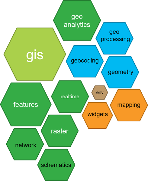
ArcGIS API for Python

- Python library for spatial analysis, mapping and GIS
- Powerful, modern and easy to use
- Powered by Web GIS
ArcGIS + Jupyter = ❤

It all starts with your GIS
In [1]:
from arcgis.gis import GIS
In [2]:
gis = GIS('https://deldev.maps.arcgis.com', 'demo_deldev', 'P@ssword123')
In [3]:
enterprise = GIS('https://python.playground.esri.com/portal', 'arcgis_python', 'amazing_arcgis_123')
Search for content
In [4]:
items = gis.content.search('San Diego')
In [5]:
for item in items:
    display(item)


In [6]:
trolley_stations = items[0]
sd_attractions = items[2]
Visualize layers on map widget
In [7]:
sdmap = gis.map('San Diego', zoomlevel=14)
sdmap
In [8]:
sdmap.add_layer(sd_attractions)
In [9]:
sdmap.add_layer(trolley_stations)

Which attractions are near trolley stations?
In [10]:
arcgis.env.active_gis = gis
In [11]:
from arcgis.features.use_proximity import create_buffers
from arcgis.features.manage_data import overlay_layers
In [12]:
places_to_see = overlay_layers(input_layer=sd_attractions,
                               overlay_layer=create_buffers(trolley_stations,
                                                        [0.5], units='Miles'))
In [13]:
my_map = gis.map('San Diego', zoomlevel=14)
display(my_map)
my_map.add_layer(places_to_see)
Analysis results as a table
In [14]:
df = places_to_see.query().df
df = df[['NAME', 'Title']]
df
Out[14]:
| NAME | Title | |
|---|---|---|
| 0 | Welcome to San Diego! | COUNTY CENTER/LITTLE ITALY TROLLEY STATION |
| 1 | Welcome to San Diego! | CIVIC CENTER TROLLEY STATION |
| 2 | Welcome to San Diego! | FIFTH AVENUE TROLLEY STATION |
| 3 | Welcome to San Diego! | AMERICA PLAZA TROLLEY STATION |
| 4 | Welcome to San Diego! | SANTA FE DEPOT |
| 5 | Welcome to San Diego! | SEAPORT VILLAGE TROLLEY STATION |
| 6 | Gaslamp Quarter | 12TH AND MARKET TROLLEY STATION |
| 7 | Convention Center skywalk and stairs | CONVENTION CENTER TROLLEY STATION |
| 8 | Convention Center skywalk and stairs | GASLAMP QUARTER TROLLEY STATION |
| 9 | Gaslamp Quarter | 12TH AND IMPERIAL TRANSIT CENTER |
| 10 | Gaslamp Quarter | 12TH AND IMPERIAL TRANSIT CENTER |
| 11 | Old Town San Diego State Historic Park | OLD TOWN TRANSIT CENTER |
Feature data and analysis
In [15]:
counties_item = gis.content.search('USA Counties', 'Feature Layer',
                                   outside_org=True)[5]
counties_item
Out[15]:

In [16]:
counties = counties_item.layers[0]
In [17]:
ca_counties = counties.query(where="STATE_NAME='California'")
Spatial dataframe
In [18]:
counties_df = ca_counties.df
counties_df
Out[18]:
| AGE_10_14 | AGE_15_19 | AGE_20_24 | AGE_25_34 | AGE_35_44 | AGE_45_54 | AGE_55_64 | AGE_5_9 | AGE_65_74 | AGE_75_84 | ... | POP10_SQMI | POP12_SQMI | POP2010 | POP2012 | RENTER_OCC | SQMI | STATE_NAME | VACANT | WHITE | SHAPE | |
|---|---|---|---|---|---|---|---|---|---|---|---|---|---|---|---|---|---|---|---|---|---|
| 0 | 68473 | 72493 | 65339 | 122046 | 108500 | 108479 | 77285 | 68694 | 43502 | 23473 | ... | 102.9 | 104.282870 | 839631 | 851089 | 101782 | 8161.35 | California | 29757 | 499766 | {'rings': [[[-13119789.4732166, 4272899.442060... |
| 1 | 11324 | 11356 | 13158 | 25589 | 21878 | 20282 | 12924 | 11564 | 6844 | 3809 | ... | 109.9 | 111.427421 | 152982 | 155039 | 18904 | 1391.39 | California | 2634 | 83027 | {'rings': [[[-13342775.4280577, 4356085.351079... |
| 2 | 3888 | 4190 | 3362 | 6603 | 7095 | 10255 | 10625 | 3574 | 6553 | 3502 | ... | 48.6 | 49.082334 | 64665 | 65253 | 9076 | 1329.46 | California | 8944 | 52033 | {'rings': [[[-13667224.3154792, 4696180.986610... |
| 3 | 1853 | 2107 | 2831 | 6337 | 5513 | 5447 | 4113 | 1595 | 1984 | 1041 | ... | 7.4 | 7.422856 | 34895 | 35039 | 3468 | 4720.42 | California | 2652 | 25532 | {'rings': [[[-13418482.3589672, 5039533.376017... |
| 4 | 678845 | 753630 | 752788 | 1475731 | 1430326 | 1368947 | 1013156 | 633690 | 568470 | 345603 | ... | 2402.3 | 2423.264150 | 9818605 | 9904341 | 1696455 | 4087.19 | California | 203872 | 4936599 | {'rings': [[[-13149469.25, 3995666.625], [-131... |
| 5 | 11755 | 12224 | 11032 | 20562 | 19167 | 19291 | 15833 | 11756 | 9868 | 5468 | ... | 70.1 | 71.065672 | 150865 | 153025 | 15591 | 2153.29 | California | 5823 | 94456 | {'rings': [[[-13337486.1875, 4418437.5625], [-... |
| 6 | 14241 | 12798 | 10308 | 24836 | 36478 | 42055 | 40088 | 15481 | 23211 | 12425 | ... | 480.2 | 486.100489 | 252409 | 255509 | 38573 | 525.63 | California | 8004 | 201963 | {'rings': [[[-13691681.78125, 4611910], [-1369... |
| 7 | 987 | 1026 | 827 | 1651 | 1828 | 3232 | 3283 | 821 | 2253 | 1186 | ... | 12.5 | 12.613887 | 18251 | 18455 | 2466 | 1463.07 | California | 2495 | 16103 | {'rings': [[[-13364133.625, 4464660.5], [-1336... |
| 8 | 5390 | 5613 | 4874 | 10704 | 10268 | 12476 | 14417 | 5259 | 7556 | 3983 | ... | 25.0 | 25.083070 | 87841 | 88094 | 14344 | 3512.09 | California | 5378 | 67218 | {'rings': [[[-13752510.6332503, 4689126.202854... |
| 9 | 22115 | 24451 | 20195 | 35060 | 31967 | 31007 | 22645 | 22167 | 13205 | 7717 | ... | 129.4 | 129.897434 | 255793 | 256841 | 34446 | 1977.26 | California | 8056 | 148381 | {'rings': [[[-13401606.6535612, 4527640.672262... |
| 10 | 602 | 604 | 422 | 904 | 1062 | 1444 | 1634 | 564 | 1108 | 570 | ... | 2.3 | 2.329272 | 9686 | 9791 | 1278 | 4203.46 | California | 1128 | 8084 | {'rings': [[[-13502305.9151577, 5160605.154186... |
| 11 | 770 | 820 | 1118 | 2253 | 1909 | 2342 | 1892 | 828 | 922 | 376 | ... | 4.5 | 4.604771 | 14202 | 14418 | 2540 | 3131.10 | California | 8144 | 11697 | {'rings': [[[-13305023.4194887, 4674333.605046... |
| 12 | 29037 | 32624 | 32481 | 62077 | 54820 | 53254 | 43218 | 30577 | 22921 | 14744 | ... | 125.2 | 126.859300 | 415057 | 420465 | 61869 | 3314.42 | California | 13102 | 230717 | {'rings': [[[-13520087.6809747, 4283419.790017... |
| 13 | 9040 | 9473 | 8289 | 16755 | 17851 | 19932 | 17843 | 8576 | 10522 | 6576 | ... | 173.1 | 172.308609 | 136484 | 135855 | 18279 | 788.44 | California | 5883 | 97525 | {'rings': [[[-13620149.8647747, 4698245.425388... |
| 14 | 5798 | 6091 | 4439 | 9654 | 10485 | 15826 | 17982 | 4950 | 10598 | 5817 | ... | 101.3 | 102.564339 | 98764 | 99951 | 11637 | 974.52 | California | 11063 | 90233 | {'rings': [[[-13430887.9145485, 4796964.419990... |
| 15 | 210195 | 227689 | 213601 | 413528 | 439043 | 444185 | 321854 | 198769 | 187454 | 112703 | ... | 3767.3 | 3822.423158 | 3010232 | 3054269 | 404468 | 799.04 | California | 56126 | 1830758 | {'rings': [[[-13102225.2452518, 3956360.076072... |
| 16 | 24986 | 24298 | 17936 | 39173 | 46565 | 53339 | 44118 | 23604 | 28990 | 17318 | ... | 232.0 | 237.083491 | 348432 | 356116 | 38404 | 1502.07 | California | 20021 | 290977 | {'rings': [[[-13476451.8800501, 4701753.649061... |
| 17 | 1022 | 1293 | 930 | 1698 | 1908 | 3226 | 3925 | 968 | 2534 | 1196 | ... | 7.7 | 7.653217 | 20007 | 20000 | 2742 | 2613.28 | California | 6589 | 17797 | {'rings': [[[-13508234.9379716, 4931510.762992... |
| 18 | 177644 | 187125 | 154572 | 282429 | 293305 | 292738 | 213739 | 167065 | 140598 | 85796 | ... | 299.8 | 305.044946 | 2189641 | 2227789 | 224048 | 7303.15 | California | 114447 | 1335147 | {'rings': [[[-12741132.318736, 4039524.4052527... |
| 19 | 99820 | 105680 | 101908 | 206646 | 190835 | 200536 | 155637 | 98112 | 83295 | 52193 | ... | 1427.5 | 1441.219615 | 1418788 | 1432457 | 218463 | 993.92 | California | 41987 | 815151 | {'rings': [[[-13527725.8606631, 4683984.725626... |
| 20 | 4709 | 4534 | 3507 | 6931 | 7621 | 8249 | 5940 | 4326 | 2978 | 1684 | ... | 39.7 | 40.634754 | 55269 | 56501 | 5878 | 1390.46 | California | 1065 | 35181 | {'rings': [[[-13519779.8682629, 4437538.523669... |
| 21 | 168792 | 179627 | 159908 | 282091 | 272949 | 277294 | 197043 | 157368 | 103495 | 56979 | ... | 101.2 | 102.560224 | 2035210 | 2062041 | 228045 | 20105.66 | California | 88019 | 1153161 | {'rings': [[[-12873899.6217711, 4274386.336024... |
| 22 | 198716 | 225095 | 270750 | 470922 | 420563 | 430774 | 329616 | 194029 | 180554 | 116911 | ... | 730.6 | 740.583699 | 3095313 | 3137431 | 495840 | 4236.43 | California | 77921 | 1981442 | {'rings': [[[-13049824.1875, 3866990.3125], [-... |
| 23 | 26299 | 34606 | 60618 | 168120 | 133682 | 111807 | 96596 | 28462 | 54322 | 38029 | ... | 16995.3 | 17398.353736 | 805235 | 824334 | 222165 | 47.38 | California | 31131 | 390387 | {'rings': [[[-13692698.0128538, 4536182.208346... |
| 24 | 56165 | 58382 | 48451 | 90815 | 90738 | 91839 | 68697 | 54810 | 38530 | 22709 | ... | 480.4 | 482.643869 | 685306 | 688477 | 87737 | 1426.47 | California | 18748 | 349287 | {'rings': [[[-13461587.15625, 4542560.5], [-13... |
| 25 | 14201 | 21727 | 27342 | 32108 | 29752 | 39253 | 37116 | 13773 | 21187 | 13531 | ... | 81.2 | 81.815416 | 269637 | 271619 | 41096 | 3319.90 | California | 15299 | 222756 | {'rings': [[[-13391141.9702506, 4153438.912972... |
| 26 | 42463 | 41249 | 40098 | 99334 | 108100 | 110669 | 89187 | 44729 | 49985 | 30973 | ... | 1573.2 | 1591.217045 | 718451 | 726677 | 104727 | 456.68 | California | 13194 | 383535 | {'rings': [[[-13618773.8429706, 4454508.553190... |
| 27 | 26626 | 38009 | 43026 | 57692 | 50478 | 54998 | 45015 | 26303 | 26776 | 18532 | ... | 154.1 | 154.042992 | 423895 | 423800 | 67277 | 2751.18 | California | 10730 | 295124 | {'rings': [[[-13252178.8386541, 3957202.320497... |
| 28 | 113570 | 114544 | 113117 | 269566 | 278369 | 263594 | 185546 | 121928 | 106521 | 62948 | ... | 1372.2 | 1401.071327 | 1781642 | 1819137 | 255906 | 1298.39 | California | 27716 | 836616 | {'rings': [[[-13539883.40625, 4506615.125], [-... |
| 29 | 15347 | 21834 | 24391 | 33749 | 33075 | 38777 | 35935 | 15071 | 15874 | 8668 | ... | 587.3 | 587.522944 | 262382 | 262470 | 40126 | 446.74 | California | 10121 | 190208 | {'rings': [[[-13605624.0035457, 4469113.194639... |
| 30 | 11394 | 12439 | 11003 | 19957 | 19567 | 26585 | 25506 | 10537 | 16551 | 9446 | ... | 46.1 | 46.480517 | 177223 | 178831 | 25069 | 3847.44 | California | 6967 | 153726 | {'rings': [[[-13601584.4375, 4921950.875], [-1... |
| 31 | 156 | 170 | 118 | 243 | 335 | 571 | 693 | 131 | 396 | 207 | ... | 3.4 | 3.353291 | 3240 | 3226 | 417 | 962.04 | California | 846 | 3022 | {'rings': [[[-13454256.3396814, 4832637.658362... |
| 32 | 2726 | 2757 | 2178 | 4277 | 4536 | 6910 | 7851 | 2410 | 4941 | 2689 | ... | 7.1 | 7.120891 | 44900 | 45200 | 6876 | 6347.52 | California | 4405 | 38030 | {'rings': [[[-13622860.3990647, 5162398.136903... |
| 33 | 28575 | 30484 | 28761 | 54914 | 54423 | 63950 | 51227 | 27311 | 25997 | 14838 | ... | 464.6 | 470.005058 | 413344 | 418187 | 52110 | 889.75 | California | 10940 | 210751 | {'rings': [[[-13568166.783698, 4655864.8583804... |
| 34 | 91070 | 100394 | 107049 | 228204 | 227491 | 222617 | 173502 | 94546 | 90437 | 52576 | ... | 2029.8 | 2062.402226 | 1510271 | 1534551 | 253896 | 744.06 | California | 37411 | 649122 | {'rings': [[[-13608423.59375, 4548229.5625], [... |
| 35 | 69 | 55 | 51 | 97 | 136 | 215 | 235 | 80 | 109 | 51 | ... | 1.6 | 1.543841 | 1175 | 1148 | 140 | 743.60 | California | 1263 | 881 | {'rings': [[[-13347105.1792653, 4711608.303495... |
| 36 | 29724 | 33298 | 32068 | 61297 | 60603 | 73518 | 68544 | 29263 | 35544 | 20614 | ... | 304.3 | 306.323820 | 483878 | 487061 | 73545 | 1590.02 | California | 18747 | 371412 | {'rings': [[[-13737803, 4672279], [-13737811.4... |
| 37 | 1881 | 2288 | 1648 | 3640 | 4518 | 6369 | 6796 | 1655 | 4455 | 2408 | ... | 62.9 | 63.288340 | 38091 | 38354 | 3686 | 606.02 | California | 3463 | 33149 | {'rings': [[[-13366995.6593785, 4680079.753190... |
| 38 | 41276 | 42807 | 37119 | 70194 | 66726 | 69558 | 52150 | 40013 | 29637 | 17785 | ... | 339.8 | 342.538842 | 514453 | 518549 | 65816 | 1513.84 | California | 14323 | 337342 | {'rings': [[[-13489390.53125, 4536971.875], [-... |
| 39 | 7146 | 7377 | 6286 | 12666 | 11980 | 12742 | 10105 | 7292 | 6490 | 3979 | ... | 155.7 | 157.125955 | 94737 | 95619 | 12225 | 608.55 | California | 2421 | 57749 | {'rings': [[[-13573190.9740771, 4740208.361085... |
| 40 | 12911 | 17841 | 22818 | 26681 | 23329 | 28877 | 28878 | 12439 | 17185 | 10962 | ... | 131.2 | 132.554757 | 220000 | 222350 | 36627 | 1677.42 | California | 8217 | 180096 | {'rings': [[[-13575499.4019644, 4825046.454825... |
| 41 | 2770 | 2893 | 1883 | 3608 | 4605 | 7565 | 8458 | 2239 | 5809 | 2784 | ... | 44.0 | 44.582939 | 45578 | 46212 | 4366 | 1036.54 | California | 9039 | 40522 | {'rings': [[[-13404519.90625, 4591131.28125], ... |
| 42 | 4431 | 4654 | 3656 | 7088 | 7316 | 9254 | 8258 | 4326 | 5720 | 3172 | ... | 21.4 | 21.523312 | 63463 | 63757 | 8404 | 2962.23 | California | 3220 | 51721 | {'rings': [[[-13598808.5625, 4923627.96875], [... |
| 43 | 1692 | 1773 | 1287 | 2780 | 2678 | 2767 | 2373 | 1733 | 1367 | 779 | ... | 18.5 | 18.833988 | 21419 | 21780 | 2738 | 1156.42 | California | 827 | 13854 | {'rings': [[[-13617316.5625, 4710753.59375], [... |
| 44 | 744 | 789 | 544 | 1271 | 1388 | 2326 | 2697 | 640 | 1674 | 837 | ... | 4.3 | 4.384289 | 13786 | 14063 | 1799 | 3207.59 | California | 2598 | 12033 | {'rings': [[[-13759504.3858904, 4996203.383529... |
| 45 | 38926 | 39043 | 32457 | 61859 | 54685 | 52351 | 40055 | 39950 | 22946 | 13474 | ... | 91.4 | 92.738012 | 442179 | 448724 | 53766 | 4838.62 | California | 11344 | 265618 | {'rings': [[[-13188692.1133358, 4403600.328655... |
| 46 | 74444 | 73766 | 59943 | 129643 | 148650 | 164080 | 128758 | 72285 | 70719 | 40347 | ... | 1380.9 | 1405.326067 | 1049025 | 1067570 | 123460 | 759.66 | California | 24899 | 614512 | {'rings': [[[-13573493.2050787, 4540676.361888... |
| 47 | 1718 | 1870 | 1799 | 4081 | 3832 | 4450 | 3717 | 1567 | 2153 | 1263 | ... | 28.2 | 28.298164 | 28610 | 28685 | 3793 | 1013.67 | California | 1279 | 21098 | {'rings': [[[-13813084.6919465, 5088634.913516... |
| 48 | 2920 | 3210 | 2951 | 6077 | 6018 | 8597 | 9469 | 2501 | 6187 | 3632 | ... | 24.3 | 24.304973 | 55365 | 55331 | 6685 | 2276.53 | California | 9088 | 48274 | {'rings': [[[-13428800.9375, 4559816.375], [-1... |
| 49 | 60390 | 64407 | 56183 | 105460 | 111083 | 123704 | 93476 | 56970 | 51396 | 30870 | ... | 443.4 | 444.788666 | 823318 | 825977 | 92752 | 1857.01 | California | 14775 | 565804 | {'rings': [[[-13306531.4673448, 3933240.934103... |
| 50 | 12506 | 12522 | 8958 | 17244 | 22203 | 32346 | 28116 | 11126 | 15437 | 7969 | ... | 101.4 | 102.156840 | 181058 | 182494 | 18832 | 1786.41 | California | 17936 | 156793 | {'rings': [[[-13425879.1875, 4650646.21875], [... |
| 51 | 12693 | 19318 | 27185 | 28168 | 23913 | 24830 | 20159 | 12235 | 10570 | 6227 | ... | 196.3 | 199.657989 | 200849 | 204322 | 33456 | 1023.36 | California | 4182 | 126883 | {'rings': [[[-13582749.7458224, 4711061.496504... |
| 52 | 75409 | 81306 | 75290 | 132729 | 114369 | 115052 | 88854 | 75040 | 49499 | 30304 | ... | 154.8 | 157.172588 | 930450 | 944788 | 130700 | 6011.15 | California | 26140 | 515145 | {'rings': [[[-13342158.5, 4418469.5625], [-133... |
| 53 | 2227 | 2156 | 1770 | 3510 | 3343 | 3835 | 3251 | 2115 | 2046 | 1185 | ... | 21.2 | 21.488749 | 28122 | 28516 | 3700 | 1327.02 | California | 978 | 19990 | {'rings': [[[-13575499.4019644, 4825046.454825... |
| 54 | 5547 | 5466 | 5395 | 10413 | 8875 | 9548 | 7567 | 5872 | 4181 | 2311 | ... | 112.1 | 113.153192 | 72155 | 72822 | 9839 | 643.57 | California | 3328 | 49332 | {'rings': [[[-13471845.3690452, 4805888.527145... |
| 55 | 7242 | 9531 | 11878 | 19995 | 15068 | 18749 | 19373 | 7324 | 9671 | 5489 | ... | 37.6 | 38.062105 | 134623 | 136375 | 25211 | 3582.96 | California | 5528 | 109920 | {'rings': [[[-13849505.9835925, 4929991.129878... |
| 56 | 14536 | 15047 | 13188 | 24197 | 22941 | 22497 | 16603 | 13841 | 9791 | 6356 | ... | 38.9 | 39.744560 | 174528 | 178091 | 21661 | 4480.89 | California | 6941 | 102553 | {'rings': [[[-12773677.4661567, 3953028.899364... |
| 57 | 1134 | 1087 | 865 | 2020 | 1969 | 2961 | 2920 | 985 | 1818 | 1196 | ... | 1.8 | 1.819773 | 18546 | 18611 | 2928 | 10227.10 | California | 1429 | 13741 | {'rings': [[[-13126868.6074171, 4504168.346584... |
58 rows × 52 columns
Pandorable (attribute and spatial) selections
In [19]:
sd_county = counties_df[counties_df.NAME == 'San Diego']
In [20]:
# Attribute query
sd_county.POP2012.iloc[0]
Out[20]:
3137431
In [21]:
# query the shape of San Diego county and set it's spatial reference
sd_geom = sd_county.SHAPE.iloc[0]
sd_geom.spatial_reference = counties.container.properties.spatialReference
In [22]:
m = gis.map('San Diego', zoomlevel=7)
m.draw(sd_geom)
m
Exploratory data analysis
In [23]:
%matplotlib inline
plotdf = counties_df.set_index('NAME')
plotdf.POP2012.plot(kind='bar', x='NAME', figsize=(15,5))
Out[23]:
<matplotlib.axes._subplots.AxesSubplot at 0x1a0896806a0>

Smart Mapping
In [24]:
ca_map = gis.map("California")
ca_map
In [25]:
ca_map.add_layer(counties, {
                             "definition_expression": "STATE_NAME='California'",
                             "renderer": "ClassedColorRenderer",
                             "field_name": "POP2012"
                            })
Big-data analysis (GeoAnalytics)

Analyse crimes in Houston, TX

In [26]:
houston_gis = GIS('https://dev003246.esri.com/portal', USERNAME, PASSWORD, verify_cert=False)
Attach data
In [27]:
datastores = arcgis.geoanalytics.get_datastores()
datastores.add_bigdata('Houston_crime_yearly',
                       r'\\teton\atma_shared\datasets\HoustonCrime')
Big Data file share exists for Houston_crime_yearly
Out[27]:
<Datastore title:"/bigDataFileShares/Houston_crime_yearly" type:"bigDataFileShare">
In [28]:
houston_yearly = houston_gis.content.search('Houston_crime_yearly',
                                            'big data file share')[0]
houston_yearly
Out[28]:

In [29]:
houston_yearly = houston_gis.content.search('Houston_crime_yearly',
                                            'big data file share')[0]
In [30]:
houston_yearly.layers
Out[30]:
[<Layer url:"https://dev003247.esri.com/gax/rest/services/DataStoreCatalogs/bigDataFileShares_Houston_crime_yearly/BigDataCatalogServer/houstoncrime2010">,
 <Layer url:"https://dev003247.esri.com/gax/rest/services/DataStoreCatalogs/bigDataFileShares_Houston_crime_yearly/BigDataCatalogServer/houstoncrime2011">,
 <Layer url:"https://dev003247.esri.com/gax/rest/services/DataStoreCatalogs/bigDataFileShares_Houston_crime_yearly/BigDataCatalogServer/houstoncrime2012">,
 <Layer url:"https://dev003247.esri.com/gax/rest/services/DataStoreCatalogs/bigDataFileShares_Houston_crime_yearly/BigDataCatalogServer/houstoncrime2013">,
 <Layer url:"https://dev003247.esri.com/gax/rest/services/DataStoreCatalogs/bigDataFileShares_Houston_crime_yearly/BigDataCatalogServer/houstoncrime2014">,
 <Layer url:"https://dev003247.esri.com/gax/rest/services/DataStoreCatalogs/bigDataFileShares_Houston_crime_yearly/BigDataCatalogServer/houstoncrime2015">,
 <Layer url:"https://dev003247.esri.com/gax/rest/services/DataStoreCatalogs/bigDataFileShares_Houston_crime_yearly/BigDataCatalogServer/houstoncrime2016">]
Invoke batch analytics
In [31]:
from ipywidgets import *
from arcgis.geoanalytics.analyze_patterns import find_hot_spots
arcgis.env.process_spatial_reference=32611
arcgis.env.verbose = False
houston = arcgis.geocoding.geocode('Houston, TX')[0]
In [ ]:
for category in df.Category.unique()[:-1]:
    lyrid = 0
    for year in range(2010, 2017):
        output_name='Houston_' + category.replace(' ', '_') + '_Hotspot_' + str(year)
        print('Generating ' + output_name)
        layer = houston_yearly.layers[lyrid]
        layer.filter = "Category='{}'".format(category)

        find_hot_spots(layer, bin_size=0.5, bin_size_unit='Miles',
                       neighborhood_distance=1, neighborhood_distance_unit='Miles',
                       output_name=output_name)

        lyrid = lyrid + 1
In [33]:
hotmap1 = houston_gis.map(houston, 10)
hotmap1.add_layer(houston_gis.content.search('Houston_Burglary_Hotspot_2016')[0])
hotmap2 = houston_gis.map(houston, 10)
hotmap2.add_layer(houston_gis.content.search('Houston_Auto_Theft_Hotspot_2016')[0])

hotmap1.layout=Layout(flex='1 1', padding='3px')
hotmap2.layout=Layout(flex='1 1', padding='3px')

items_layout = Layout(flex='1 1 auto', width='auto')
In [34]:
display(HBox([hotmap1, hotmap2]))
display(HBox(children=[Button(description='Burglary hot spots in 2016', layout=items_layout, button_style='danger'),
                       Button(description='Auto theft hot spots in 2016', layout=items_layout, button_style='danger')],
             layout=Layout(width='100%')))
Compare Hot Spots over time
In [35]:
maps = []
labels = []
items_layout = Layout(flex='1 1 auto', width='auto')
layout=Layout(height='300px')
In [36]:
for year in range(2014, 2017):
    layer = houston_gis.content.search('Houston_Auto_Theft_Hotspot_' + str(year))[0]
    hotspotmap = houston_gis.map(houston)
    hotspotmap.add_layer(layer)
    hotspotmap.layout=Layout(flex='1 1', padding='3px')
    maps.append(hotspotmap)
    hotspotmap.basemap='gray'
    labels.append(Button(description='Auto theft hot spots in ' + str(year),
                         layout=items_layout, button_style='danger'))

display(HBox([maps[0], maps[1], maps[2]], layout=layout))
display(HBox(children=labels, layout=Layout(width='100%')))
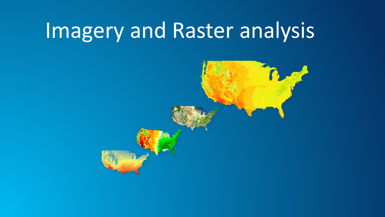
Use Landsat Imagery
In [37]:
landsat_item = gis.content.search('"Landsat Multispectral"',
                                  'Imagery Layer', outside_org=True)[0]
In [38]:
landsat_item
Out[38]:

In [39]:
landsat = landsat_item.layers[0]
Visualize imagery layers
In [40]:
imagery_map = gis.map('San Diego, CA', zoomlevel=12)
imagery_map.add_layer(landsat)
imagery_map
Code: Plot spectral profile at clicked location
In [41]:
import pandas as pd
pd.DataFrame(landsat.key_properties()['BandProperties'])
Out[41]:
| BandIndex | BandName | DatasetTag | WavelengthMax | WavelengthMin | |
|---|---|---|---|---|---|
| 0 | 0 | CoastalAerosol | MS | 450 | 430 |
| 1 | 1 | Blue | MS | 510 | 450 |
| 2 | 2 | Green | MS | 590 | 530 |
| 3 | 3 | Red | MS | 670 | 640 |
| 4 | 4 | NearInfrared | MS | 880 | 850 |
| 5 | 5 | ShortWaveInfrared_1 | MS | 1650 | 1570 |
| 6 | 6 | ShortWaveInfrared_2 | MS | 2290 | 2110 |
| 7 | 7 | Cirrus | MS | 1380 | 1360 |
In [42]:
from bokeh.models import Range1d
from bokeh.plotting import figure, show, output_notebook
from IPython.display import clear_output

output_notebook()

def handle_click(m, pt):
    m.draw(pt)

    samples = landsat.get_samples(pt, pixel_size=30)
    values = samples[0]['value']

    x = ['1','2', '3', '4', '5', '6', '7', '8']
    y = [float(int(s)/100000) for s in values.split(' ')]

    p = figure(title="Spectral Profile", x_axis_label='Spectral Bands',
               y_axis_label='Data Values', width=600, height=300)
    p.line(x, y, legend="Selected Point", line_color="red", line_width=2)
    p.circle(x, y, line_color="red", fill_color="white", size=8)
    p.set(y_range=Range1d(0, 1.0))

    clear_output()
    show(p)
In [43]:
click_map = gis.map('San Diego, CA', zoomlevel=12)
click_map.add_layer(landsat)
click_map.on_click(handle_click)
Demo: Plot spectral profile at clicked location
In [44]:
click_map
Dynamic raster processing
In [45]:
dynamic_map = gis.map('San Diego, CA', zoomlevel=12)
dynamic_map.add_layer(landsat)
dynamic_map
In [46]:
from arcgis.raster.functions import *
from IPython.display import clear_output
import time
In [111]:
for rasterfunc in landsat.properties.rasterFunctionInfos:
    clear_output()
    print(rasterfunc.name)

    dynamic_map.add_layer(apply(landsat, rasterfunc.name))
    time.sleep(2)
None
Custom raster processing using Raster Functions
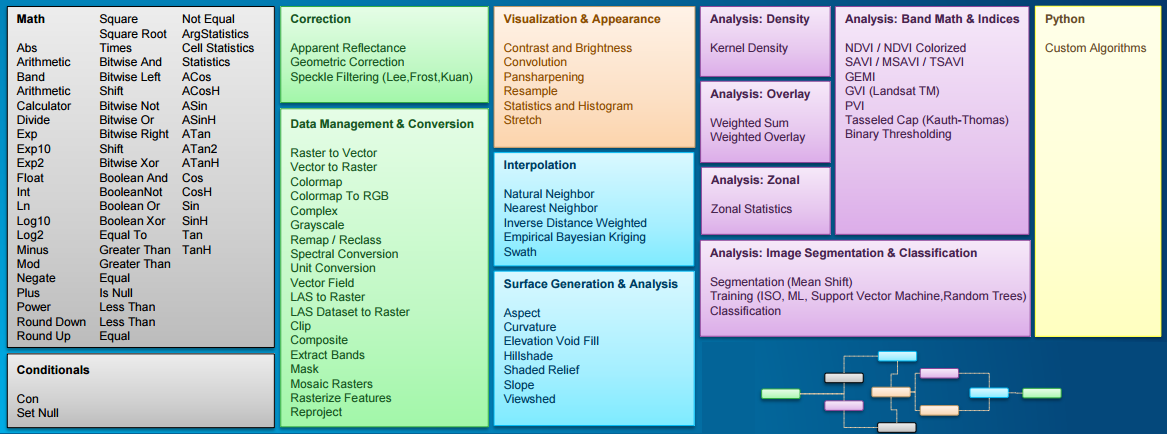
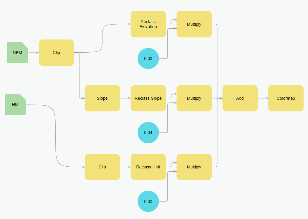
Function chain for weighted overlay analysis
In [48]:
# Digital elevation model for the US

item_dem = enterprise.content.search('elevation_270m')[0]
lyr_dem = item_dem.layers[0]
lyr_dem
Out[48]:

Human modified index
In [49]:
# Human Modified Index imagery layer
# This dataset is based on research on the degree of human modification to
# the landscape, on a scale of 0 - 1, where 0.0 indicates unmodified natural
# landscape and 1.0 indicates the landscape is completely modified by human activity.

item_hmi = enterprise.content.search('human_modification_index')[0]
lyr_hmi = item_hmi.layers[0]
lyr_hmi
Out[49]:

Set area of interest as layer's extent
In [50]:
# geocode the area of interest
from arcgis.geocoding import geocode

sd_county = geocode('San Diego County',
                    out_sr=lyr_dem.properties.spatialReference)[0]
In [51]:
# set the area of interest as the layer's extent
lyr_dem.extent = sd_county['extent']
lyr_dem
Out[51]:

Interactive raster processing in Jupyter Notebook
In [52]:
clipped_elev = clip(lyr_dem, sd_geom)
clipped_elev
Out[52]:

In [53]:
# Create a colormap for rendering the analysis results.

red_green =  [[1,  38, 115,0],[2,  86, 148,0],[3,  0x8B, 0xB5,0],[4,  0xC5, 0xDB,0],
         [5, 255, 255, 0],[6,  0xFF, 0xC3,0],[7, 0xFA, 0x8E, 0],[8,  0xF2, 0x55,0],
         [9, 0xE6, 0, 0]]
Chaining raster functions
In [54]:
output_values = [1,2,3,4,5,6,7,8,9]

colormap(remap(slope(clipped_elev,
                     slope_type='DEGREE',
                     z_factor=1),
               input_ranges=[0,1, 1,2, 2,3, 3,5, 5,7, 7,9, 9,12, 12,15, 15,100],
               output_values=output_values),
         colormap=red_green)
Out[54]:

In [55]:
colormap(remap(clip(lyr_dem, sd_geom),  # Elevation
                    input_ranges=[-90,250, 250,500, 500,750, 750,1000, 1000,1500, 1500,2000, 2000,2500, 2500,3000, 3000,5000],
                    output_values=[1,2,3,4,5,6,7,8,9]) ,
        colormap=red_green)
Out[55]:

In [56]:
lyr_hmi.extent = sd_county['extent']
colormap(remap(clip(lyr_hmi, sd_geom), # Human modified index
                     input_ranges=[0.0,0.1, 0.1,0.2, 0.2,0.3, 0.3,0.4, 0.4,0.5,0.5,0.6, 0.6,0.7, 0.7,0.8, 0.8,1.1],
                     output_values=[1,2,3,4,5,6,7,8,9]),
        colormap=red_green)
Out[56]:

Prepare input layers
In [57]:
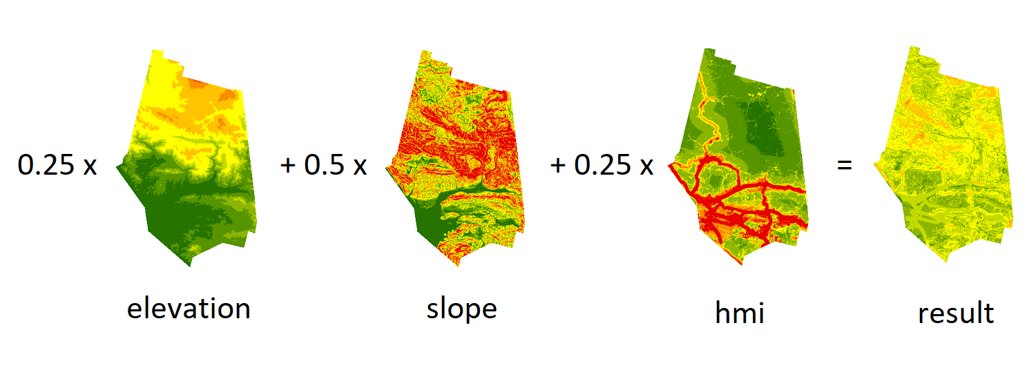
elevation = remap(lyr_dem,  # Elevation
                    [-90,250, 250,500, 500,750, 750,1000, 1000,1500, 1500,2000, 2000,2500, 2500,3000, 3000,5000],
                    output_values)
In [58]:
natural_areas = remap(lyr_hmi, # Human Modified Index
                     [0.0,0.1, 0.1,0.2, 0.2,0.3, 0.3,0.4, 0.4,0.5,0.5,0.6, 0.6,0.7, 0.7,0.8, 0.8,1.1],
                     output_values)
In [59]:
terrain = remap(slope(lyr_dem, slope_type='DEGREE', z_factor=1), # Slope
                     [0,1, 1,2, 2,3, 3,5, 5,7, 7,9, 9,12, 12,15, 15,100],
                     output_values)
Map algebra for Weighted Overlay Analysis
In [60]:
# Map algebra for the web GIS!
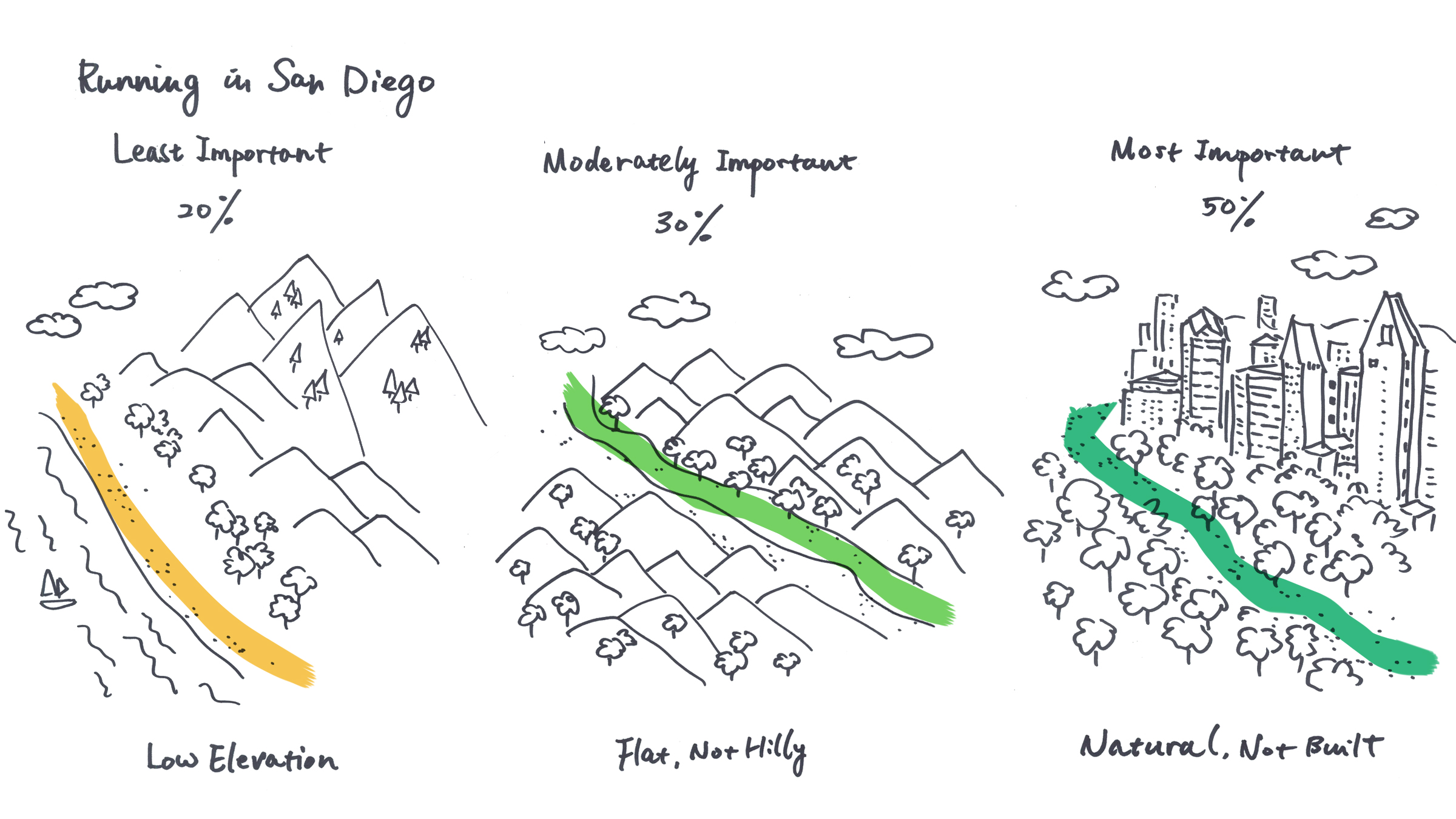
result = 0.2*elevation + 0.3*terrain + 0.5*natural_areas
In [61]:
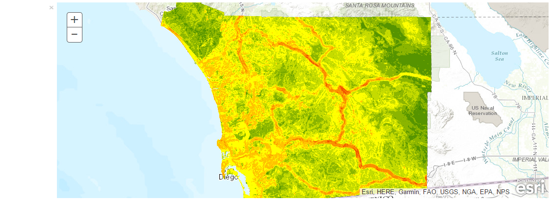
run_raster = colormap(clip(result, sd_geom), colormap=red_green)
run_raster
Out[61]:

Visualize results using map widget
In [62]:
surface_map = gis.map('San Diego, CA', zoomlevel=12)
surface_map.add_layer(run_raster)
surface_map
Persist results as an imagery layer
In [ ]:
# Generate a persistent result at source resolution using Raster Analytics
# resultlyr = weighted_overlay.save('SanDiego_PlacesToRun')
In [67]:
resultlyr = enterprise.content.search('SanDiego_PlacesToRun')[0]
In [68]:
resultlyr
Out[68]:

Results: finding solitude by applying GIS
In [69]:
enterprise_b = GIS('https://dev004546.esri.com/portal', 'rsinghRA', 'rsinghRA1', verify_cert=False)
In [81]:
with open("CCM_CostRnR.rft.xml", "r", encoding='utf-8-sig') as rft:
    raster_fn = rft.read()
In [ ]:
from arcgis.raster.analytics import generate_raster

surface = generate_raster(raster_fn, output_name='CCM_Cost_Surface')
In [ ]:
enterprise_b.content.search('CCM_Cost_Surface')
In [71]:
surface = enterprise_b.content.search('title:CCM_Cost_Surface', 'Imagery Layer')[0]
In [73]:
surface
Out[73]:

In [74]:
tank_symbol = {
  "type" : "esriPMS",
  "url" : "http://static.arcgis.com/images/Symbols/Transportation/Tank.png",
  "contentType" : "image/png",
  "width" : 19.5,
  "height" : 19.5,
  "angle" : 0,
  "xoffset" : 0,
  "yoffset" : 0
}
finish_symbol = {"angle":0,"xoffset":12,"yoffset":12,"type":"esriPMS","url":"http://static.arcgis.com/images/Symbols/Basic/CheckeredFlag.png","contentType":"image/png","width":24,"height":24}
In [75]:
from arcgis.features import FeatureSet, Feature
arcgis.env.out_spatial_reference = 4326
In [76]:
ramona = geocode("Ramona, CA", out_sr=102100)[0]
poway = geocode("Poway, CA", out_sr=102100)[0]
barona = geocode("Barona Reservation, CA", out_sr=102100)[0]

origins=FeatureSet([Feature(ramona['location']),
                    Feature(poway['location']),
                    Feature(barona['location'])])

In [77]:
from arcgis.geoprocessing import import_toolbox

ccmurl='https://maps.esri.com/apl3/rest/services/LCP/LCP/GPServer/LeastCostPath'
ccm = import_toolbox(ccmurl)
In [78]:
def find_path(m, pt):
    m.draw(pt, symbol=finish_symbol)
    paths = ccm.least_cost_path(destination=FeatureSet([Feature(pt)]),
                                origins=origins)
    m.draw(paths)
Finding least cost paths interactively
In [112]:
ccm_map = gis.map('San Vicente Reservoir', zoomlevel=10)
ccm_map.on_click(find_path)
ccm_map
In [113]:
ramona = geocode("Ramona, CA")[0]
poway = geocode("Poway, CA")[0]
barona = geocode("Barona Reservation, CA")[0]

ccm_map.draw(ramona, symbol=tank_symbol)
ccm_map.draw(poway, symbol=tank_symbol)
ccm_map.draw(barona, symbol=tank_symbol)

In [65]:
landsat.extent = {'spatialReference': {'latestWkid': 3857, 'wkid': 102100},
 'type': 'extent',
 'xmax': 4296559.143733407,
 'xmin': 4219969.241391764,
 'ymax': 3522726.823081019,
 'ymin': 3492152.0117669892}
In [66]:
landsat
Out[66]:

In [67]:
preprocessed = stretch(ndvi(landsat), stretch_type='PercentClip', min_percent=30, max_percent=70, dra=True)
preprocessed
Out[67]:

In [68]:
def count_farms():
    from skimage import feature, color
    import numpy as np
    from scipy.signal import convolve2d
    import matplotlib.pyplot as plt
    import matplotlib.image as mpimg

    img = preprocessed.export_image(size=[1200, 450],
        export_format='jpeg', save_folder='c:\\xc', save_file='saudiarabia.jpg', f='image')

    img = mpimg.imread('c:\\xc\\saudiarabia.jpg')

    bw = img.mean(axis=2)
    fig=plt.figure(figsize = (15,15))
    ax=fig.add_subplot(1,1,1)

    blobs_dog = [(x[0],x[1],x[2]) for x in feature.blob_dog(-bw,
                                                            min_sigma=4,
                                                            max_sigma=8,
                                                            threshold=0.1,
                                                            overlap=0.6)]

    blobs_dog = set(blobs_dog)

    img_blobs = color.gray2rgb(img)
    for blob in blobs_dog:
        y, x, r = blob
        c = plt.Circle((x, y), r+1, color='red', linewidth=2, fill=False)
        ax.add_patch(c)
    plt.imshow(img_blobs)
    plt.title('Center Pivot Farms')

    plt.show()
    print('Number of center pivot farms detected: ' + str(len(blobs_dog)))
In [69]:
count_farms()

Number of center pivot farms detected: 1002
In [71]:
from IPython.display import Image
In [89]:
img = r'C:\xc\Presentations\GeoPython\Watson\insulators\150362.JPG'
Image(img, width="600")
Out[89]:

In [85]:
import json
import datetime
import pandas as pd
from os import listdir
from os.path import isfile, join
from IPython.display import Image

from arcgis.gis import GIS
from arcgis.geocoding import geocode
from arcgis.features.use_proximity import plan_routes
from arcgis.features.summarize_data import join_features
Using IBM Watson Image Classifier
In [117]:
from watson_developer_cloud import VisualRecognitionV3

visual_recognition = VisualRecognitionV3('2016-05-20', api_key='f135ee67e833d45e90e2304608e0376b5a148688')

def is_broken(filepath):
    with open(filepath, 'rb') as images_file:
        car_results = visual_recognition.classify(images_file=images_file,
                                                  threshold=0.1,
                                                  classifier_ids=['BrokenInsulators'])
        print(car_results)
        classes = car_results['images'][0]['classifiers'][0]['classes']
        for cls in classes:
            if cls['class'] == 'broken':
                if float(cls['score']) > 0.5:
                    return True

        return False
In [100]:
import piexif
def get_location(filename):

    exif_dict = piexif.load(filename)

    for tag in exif_dict['GPS']:
        name = piexif.TAGS['GPS'][tag]["name"]
        value = exif_dict['GPS'][tag]

        if name == 'GPSLatitudeRef':
            gps_latitude_ref = value
        elif name == 'GPSLongitudeRef':
            gps_longitude_ref = value
        elif name == 'GPSLatitude':
            gps_latitude = value
        elif name == 'GPSLongitude':
            gps_longitude = value

    lat = _convert_to_degress(gps_latitude)
    if gps_latitude_ref != b'N':
        lat = 0 - lat

    lon = _convert_to_degress(gps_longitude)
    if gps_longitude_ref != b'E':
        lon = 0 - lon

    return lon, lat

def _convert_to_degress(val):
    """
    Helper function to convert the GPS coordinates stored in the EXIF to degress in float format
    :param value:
    :type value: exifread.utils.Ratio
    :rtype: float
    """
    d = float(val[0][0]) / float(val[0][1])
    m = float(val[1][0]) / float(val[1][1])
    s = float(val[2][0]) / float(val[2][1])

    return d + (m / 60.0) + (s / 3600.0)
In [115]:
get_location(img)
Out[115]:
(-123.05857389997222, 44.698829929999995)
In [118]:
is_broken(img)
{'images': [{'image': '', 'classifiers': [{'name': 'BrokenInsulators', 'classifier_id': 'BrokenInsulators_1382670166', 'classes': [{'score': 0.567984, 'class': 'broken'}]}]}], 'images_processed': 1, 'custom_classes': 1}
Out[118]:
True
Integration workflow
In [79]:
locations = []
path = r'C:\xc\Presentations\GeoPython\Watson\insulators'

# find locations of broken insulators
for file in listdir(path):
    filepath = path + '\\' + file
    if is_broken(filepath):
        locations.append(get_location(filepath))

# import into ArcGIS as a layer
df = pd.DataFrame.from_records(locations)
df.columns = ['x', 'y']
broken_insulators = gis.content.import_data(df)
In [104]:
locations = []
path = r'C:\xc\Presentations\GeoPython\Watson\insulators'

# find locations of broken insulators
for file in listdir(path):
    filepath = path + '\\' + file
    if True: #is_broken(filepath):
        locations.append(get_location(filepath))

# import into ArcGIS as a layer
df = pd.DataFrame.from_records(locations)
df.columns = ['x', 'y']
broken_insulators = gis.content.import_data(df)
In [105]:
arcgis.env.active_gis = gis
start_location = geocode('2715 Tepper Ln NE, Keizer, OR 97303')[0]
start_time = datetime.datetime(2017, 5, 31, 9, 0)
In [106]:
# get layer of transmission towers
towers = gis.content.search('BPA_TransmissionStructures', 'Feature Layer', outside_org=True)[0]

# find transmission towers near image locations
destinations = join_features(towers, broken_insulators,
                             "withindistance", 0.1, "Miles")

# plan and sequence routes for maintenance
routes = plan_routes(destinations, 2, 15,
                     start_time, start_location, stop_service_time=30)
Input field [OID] was not mapped to a field in the network analysis class "Orders".
Input field [OID] was not mapped to a field in the network analysis class "Depots".
In [107]:
def show_map():
    webmap = gis.content.get('4a24e5829d174732bc04f16de83eaffe')
    powermap = gis.map(webmap)
    display(powermap)
    powermap.height ='600px'
    powermap.draw(start_location, {"title": "Start location", "content": "Bonneville Power Administration"})
    return powermap
In [109]:
powermap = show_map()
In [110]:
powermap.basemap = 'dark-gray'

powermap.add_layer(broken_insulators)
powermap.add_layer(routes['routes_layer'])
powermap.add_layer(routes['assigned_stops_layer'])
In [114]:
powermap.zoom = 9
Try it out!
install: conda install -c esri arcgis
github repo: https://github.com/esri/arcgis-python-api
website: https://developers.arcgis.com/python
We're hiring :)