Burgers' equation
%matplotlib inline
%config InlineBackend.figure_format = 'svg'
import matplotlib as mpl
mpl.rcParams['font.size'] = 8
figsize =(8,4)
mpl.rcParams['figure.figsize'] = figsize
import matplotlib.pyplot as plt
import numpy as np
from ipywidgets import interact
from ipywidgets import widgets
from utils import riemann_tools
from exact_solvers import burgers
import seaborn as sns
sns.set_style('white',{'legend.frameon':'True'});
#sns.set_context('paper')
In this chapter we study another scalar nonlinear conservation law: Burgers' equation. Burgers' equation models momentum transport in a fluid of uniform density and pressure, and it is the simplest equation that captures some key features of gas dynamics. It has been used extensively for developing both theory and numerical methods, and will allow us to further explore the Riemann problem for nonlinear conservation laws. \begin{align} q_t + \left(\frac{1}{2}q^2\right)_x = 0. \label{burgers0} \end{align}
Shock formation
Burgers' equation is a scalar conservation law with the nonlinear flux term $f(q)=q^2/2$. The quasilinear form is obtained by applying the chain rule to differentiate the flux term:
\begin{align*}
q_t + qq_x = 0.
\end{align*}
This equation looks very similar to an advection equation with the exception that the advection speed is given by the value $q$. This is similar to the traffic flow equation but with a different flux. The nonlinearity in the Burgers flux term is essentially the same as in the momentum conservation equation in fluid dynamics, so studying its dynamics provides a guideline to understand more complex fluid dynamics.
One way to interpret this equation is to imagine that $q$ is the height of a water wave as it approaches the beach. The equation tells us that peak of the wave propagates faster than the trough. In the next figure, we show a solution at two different times for to illustrate this behavior.
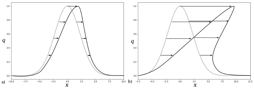
Notice that at first $q$ remains univalued for every $x$. However, after some time the crest of the wave overtakes the leading edge. After this time, we obtain a triple-valued solution. The first time this overtaking happens is referred to as the breaking time -- a reference to waves breaking on the beach. It is also the point where the conservation law, in its differential form, breaks down and where the characteristics cross each other for the first time. As we learned in Traffic_flow.ipynb, when characteristics cross, a shock wave forms. Mathematically, imposing a shock will avoid the problem of the solution being multivalued. Where should the shock be located?
If we replace part of the multivalued solution interval with a shock, some mass will be removed (area A1 in the figure below) and some mass will be added (area A2 in the figure below). In order to maintain conservation of the integral of $q$, the shock must be placed so that these two areas are equal:
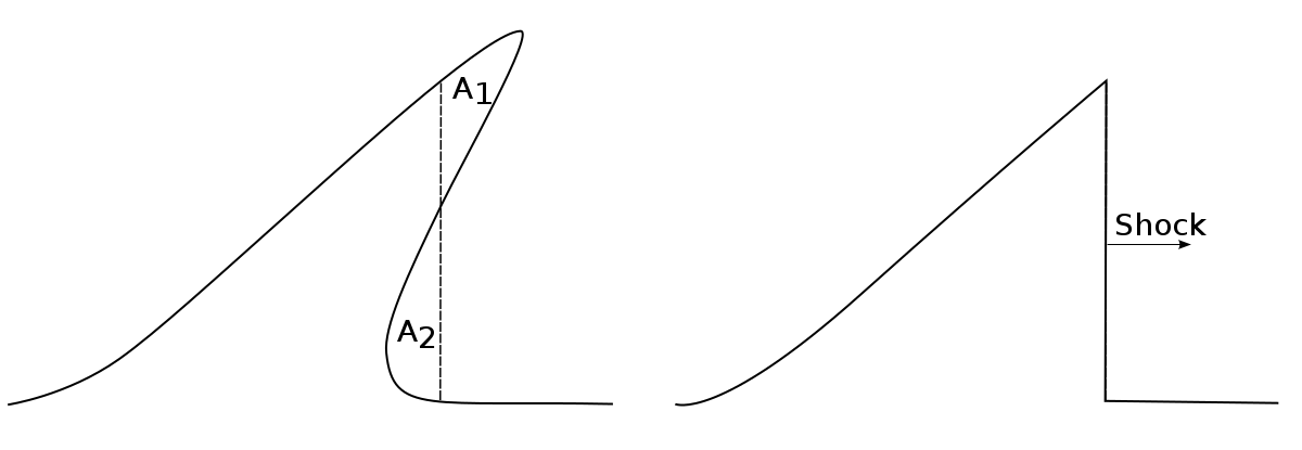
This geometric reasoning provides a nice intuition for the shock location, but is cumbersome in practice. To determine the path of the shock we can again use the Rankine-Hugoniot jump condition, derived in Traffic_flow.ipynb. Since the flux for Burgers' equation is $f(q) = q^2/2$, we have
\begin{align*}
s(q_r-q_l) & = f(q_r) - f(q_l)\\
& = \frac{1}{2} (q_r^2 - q_l^2) \\
\Rightarrow \ \ \ \ s &= \frac{1}{2}(q_l + q_r).
\end{align*}
Here $q_l, q_r$ denote the solution values just to the left and right of the shock. In general (as in the image above) these states will not be constant and the speed of a shock will change in time.
Shock solution
For Burgers' equation, as for the traffic model (or any scalar hyperbolic conservation law with a convex flux function), the solution of the Riemann problem will always consist of one wave, which may be either a shock or a rarefaction. The analysis above already yields the solution to the Riemann problem in the case that the resulting wave is a shock. The entropy condition tells us that a shock will form when $f'(q_l) > f'(q_r)$; i.e. when $q_l>q_r$. In this case the solution is
\begin{align*}
q(x,t) =
\begin{cases}
q_l \quad \text{if} \ \ x/t<s \\
q_r \quad \text{if} \ \ x/t>s.
\end{cases}
\end{align*}
We will now plot the solution of the Burgers' equation when shocks are formed, i.e. when $q_l>q_r$. We first define an interactive plotting function for the exact solver and then we choose the initial conditions and plot the solution.
def plot_riemann_solution(ql, qr):
    states, speeds, reval, wave_type = burgers.exact_riemann_solution(ql ,qr)

    plot_function = riemann_tools.make_plot_function(states, speeds, reval, wave_type, layout='horizontal',
                                                    variable_names=['q'],
                                                    plot_chars=[burgers.speed])

    return interact(plot_function, t=widgets.FloatSlider(value=0.0,min=0,max=1.0),
                    which_char=widgets.Checkbox(value=True,description='Show characteristics'));
ql = 5.0
qr = 1.0
plot_riemann_solution(ql,qr);
Rarefaction wave
In the previous figure with the hump as initial condition, we observed that a shock formed on the right side of the hump. However, on the left side, the characteristics spread out and will never cross. This part of the solution is therefore a rarefaction wave. This is the kind of behavior we will observe in the solution of the Riemann problem when $q_l<q_r$.
In the next figure, we consider such a Riemann problem. As time evolves, a rarefaction forms following the advection speed $q$ given by the quasi-linear equation. Therefore, for time $t$, the solution must propagate a distance $x=qt$, so the solution along the rarefaction is then $q = x/t$. As $q_l<q_r$, the smallest and largest displacements are given by $q_l t$ and $q_r t$, respectively.
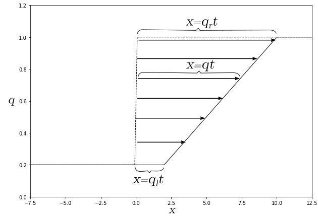
The full rarefaction solution for the Burgers' Riemann problem is then simply given by \begin{align*} q(x,t) = \begin{cases} q_l, \quad \text{for} \ \ x<q_l t \\ \frac{x}{t}, \quad \text{for} \ \ q_l t \le x \le q_r t \\ q_r, \quad \text{for} \ \ x>q_r t. \end{cases} \end{align*}
As we will see in the next chapter, the rarefaction solution is always a self-similar solution. This means that it can be expressed as a function of the ratio between position and time $q(x,t) = \tilde{q}(x/t)$, so it remains the same when rescaling both $x$ and $t$ by the same factor. This is a consequence of $q$ being the same along the characteristic in the rarefaction fan. In the Burgers' equation, the form of the rarefaction is particularly simple since the advection speed is simply $q$.
Rarefaction solution
In the figure below, we plot solutions of the Riemann problem with $q_l<q_r$. In these cases, we will always observe a rarefaction.
ql = 2.0
qr = 4.0
plot_riemann_solution(ql,qr);
Weak solutions
As we mentioned before, the differential form of the equation breaks down in the presence of shocks/discontinuities.However, the integral form of the conservation law remains valid. We will derive a specific form of the integral conservation law that is particularly useful to prove mathematical results. We first intergate the conservation law $q_t+f(q)_x=0$ from from $x=x_1$ to $x=x_2$ and $t=t_1$ to $t=t_2$
\begin{align} \int_{t_1}^{t_2}\int_{x_1}^{x_2} [q_t+f(q)_x] dx dt = 0, \label{eq:Burgersintclaw} \end{align}where $f(q)=q^2/2$ for Burgers' equation. However, this derivation is general and apply to all nonlinear scalar conservation laws. This equation can be simply rewritten in terms of a function $\phi(x,t)$ with compact support in $[x_1,x_2]x[t_1,t_2]$ (1 in this region, zero elsewhere),
\begin{align*} \int_{0}^{\infty}\int_{-\infty}^{\infty} [q_t+f(q)_x]\phi(x,t) dx dt = 0. \end{align*}Integrating by parts we obtain
\begin{align*} \int_{0}^{\infty}\int_{-\infty}^{\infty} [q\phi_t+f(q)\phi_x] dx dt = -\int_{-\infty}^{\infty}q(x,0)\phi(x,0)dx, \end{align*}where now the derivative are in $\phi(x,t)$ and not in $q$ of $f(q)$, so the equation still makes sense for discontinuous $q$. The function $q(x,t)$ is a weak solution of the conservation law if this equation holds for all functions $\phi(x,t)$ that are continuously differentiable and with compact support (bump functions). Note this rules out the original interval chosen in Eq. \ref{eq:Burgersintclaw} since its $\phi$ would not be smooth. However, we can approximate this function arbitrarily well by a smooth function. Any weak solution is a solution of any form of the integral conservation law and viceversa.
The concept of weak solutions are helpful to do mathematical proofs and manipulations. Actually, all the solution previously derived in this chapter are weak solutions of Burgers' equation. However, there is a caveat; weak solutions are not unique.
An unphysical weak solution
We previously mentioned that for Burgers' equation, when $q_l<q_r$, we expect a rarefaction to be correct solution. However, we used our physical intuiton from the characteristics and the advection equation to solve it. Nonetheless, we could assume the solution has a shock/discontinuity and by using the equation in the form of a conservation law derive the Rankine-Hugoniot as previously done. This is mathematically correct and one obtains the same relation as before $s = (q_l + q_r)/2$ for the shock speed, so the solution is simply
\begin{align*} q(x,t) = \begin{cases} q_l \quad \text{if} \ \ x/t<s \\ q_r \quad \text{if} \ \ x/t>s. \end{cases} \end{align*}This unphysical solution is also refered to as expansion shock, and it is also a weak solution to the Burgers' equation. In the next figure, we plot this weak solution.
def plot_unphysical_weak_solution(ql, qr):
    states, speeds, reval, wave_type = burgers.unphysical_riemann_solution(ql ,qr)

    plot_function = riemann_tools.make_plot_function(states, speeds, reval, wave_type, layout='horizontal',
                                                    variable_names=['q'],
                                                    plot_chars=[burgers.speed])

    return interact(plot_function, t=widgets.FloatSlider(value=0.0,min=0,max=1.0),
                    which_char=widgets.Checkbox(value=True,description='Show characteristics'));
ql = 1.0
qr = 5.0
plot_unphysical_weak_solution(ql,qr);
Note the solution is given by a shock, even though $q_l<q_r$. From the characteristics, it is clear that the correct solution should be a rarefaction. In order to be able to specify which of the weak solutions is physically correct, we need to derive a mathematical condition from our physical intutiton gained from oberving the behavior of the characteristics. This condition will be the entropy condition, and it will be explored in future chapters.
Examples
We can now explore a few more examples that are representative of phenomena we will observe in more complicated systems, as well as a full interactive example.
Example 1: Symmetric rarefaction
Symmetric rarefactions happen where the characteristic waves spread equally on opposite directions around the origin, and we will observe them in many of the nonlinear systems presented in other chapters. This means there is a point in the center where $q$ (momentum) is effectively zero for all times.
ql = -4.0
qr = 4.0
plot_riemann_solution(ql,qr);
Example 2: Full interactive solution
def plot_riemann(q_l,q_r,t,x_range=1):
    states, speeds, reval, wave_types = \
            burgers.exact_riemann_solution(q_l,q_r)
    ax = riemann_tools.plot_riemann(states,speeds,reval,
                                    wave_types,t=t,
                                    t_pointer=0,extra_axes=True,
                                    variable_names=['q'],
                                    xmax=x_range);
    riemann_tools.plot_characteristics(reval,burgers.speed,axes=ax[0])
    burgers.plot_trajectories(q_l,q_r,ax[2],t=t,xmax=x_range);
    ax[1].set_ylim(-0.05,1.05)
    for a in ax:
        a.set_xlim(-x_range,x_range)
    plt.show()
burgers.plot_interactive_riemann(plot_riemann)
Example 3:Three state solution?