Decision tree for classification¶

A Summary of lecture "Machine Learning with Tree-Based Models in Python

", via datacamp

toc: true
badges: true
comments: true
author: Chanseok Kang
categories: [Python, Datacamp, Machine_Learning]
image: images/decision-boundary.png

In [1]:

import pandas as pd
import numpy as np
import matplotlib.pyplot as plt
import seaborn as sns

Decision tree for classification¶

Classification-tree
- Sequence of if-else questions about individual features.
- Objective: infer class labels
- Able to caputre non-linear relationships between features and labels
- Don't require feature scaling(e.g. Standardization)
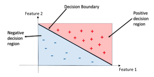
Decision Regions
- Decision region: region in the feature space where all instances are assigned to one class label
- Decision Boundary: surface separating different decision regions

decision region

Train your first classification tree¶

In this exercise you'll work with the Wisconsin Breast Cancer Dataset from the UCI machine learning repository. You'll predict whether a tumor is malignant or benign based on two features: the mean radius of the tumor (radius_mean) and its mean number of concave points (concave points_mean).

Preprocess¶

In [3]:

wbc = pd.read_csv('./dataset/wbc.csv')
wbc.head()

Out[3]:

	id	diagnosis	radius_mean	texture_mean	perimeter_mean	area_mean	smoothness_mean	compactness_mean	concavity_mean	concave points_mean	...	texture_worst	perimeter_worst	area_worst	smoothness_worst	compactness_worst	concavity_worst	concave points_worst	symmetry_worst	fractal_dimension_worst	Unnamed: 32
0	842302	M	17.99	10.38	122.80	1001.0	0.11840	0.27760	0.3001	0.14710	...	17.33	184.60	2019.0	0.1622	0.6656	0.7119	0.2654	0.4601	0.11890	NaN
1	842517	M	20.57	17.77	132.90	1326.0	0.08474	0.07864	0.0869	0.07017	...	23.41	158.80	1956.0	0.1238	0.1866	0.2416	0.1860	0.2750	0.08902	NaN
2	84300903	M	19.69	21.25	130.00	1203.0	0.10960	0.15990	0.1974	0.12790	...	25.53	152.50	1709.0	0.1444	0.4245	0.4504	0.2430	0.3613	0.08758	NaN
3	84348301	M	11.42	20.38	77.58	386.1	0.14250	0.28390	0.2414	0.10520	...	26.50	98.87	567.7	0.2098	0.8663	0.6869	0.2575	0.6638	0.17300	NaN
4	84358402	M	20.29	14.34	135.10	1297.0	0.10030	0.13280	0.1980	0.10430	...	16.67	152.20	1575.0	0.1374	0.2050	0.4000	0.1625	0.2364	0.07678	NaN

5 rows × 33 columns

In [4]:

X = wbc[['radius_mean', 'concave points_mean']]
y = wbc['diagnosis']
y = y.map({'M':1, 'B':0})

In [5]:

from sklearn.model_selection import train_test_split

X_train, X_test, y_train, y_test = train_test_split(X, y, test_size=0.2, random_state=1)

In [6]:

from sklearn.tree import DecisionTreeClassifier

# Instantiate a DecisionTreeClassifier 'dt' with a maximum depth of 6
dt = DecisionTreeClassifier(max_depth=6, random_state=1)

# Fit dt to the training set
dt.fit(X_train, y_train)

# Predict test set labels
y_pred = dt.predict(X_test)
print(y_pred[0:5])

[1 0 0 1 0]

Evaluate the classification tree¶

Now that you've fit your first classification tree, it's time to evaluate its performance on the test set. You'll do so using the accuracy metric which corresponds to the fraction of correct predictions made on the test set.

In [7]:

from sklearn.metrics import accuracy_score

# Predict test set labels
y_pred = dt.predict(X_test)

# Compute test set accuracy
acc = accuracy_score(y_test, y_pred)
print("Test set accuracy: {:.2f}".format(acc))

Test set accuracy: 0.89

Logistic regression vs classification tree¶

A classification tree divides the feature space into rectangular regions. In contrast, a linear model such as logistic regression produces only a single linear decision boundary dividing the feature space into two decision regions.

Helper function¶

In [8]:

from mlxtend.plotting import plot_decision_regions

def plot_labeled_decision_regions(X,y, models):
    '''Function producing a scatter plot of the instances contained 
    in the 2D dataset (X,y) along with the decision 
    regions of two trained classification models contained in the
    list 'models'.
    
    Parameters
    ----------
    X: pandas DataFrame corresponding to two numerical features 
    y: pandas Series corresponding the class labels
    models: list containing two trained classifiers 
    
    '''
    if len(models) != 2:
        raise Exception('''Models should be a list containing only two trained classifiers.''')
    if not isinstance(X, pd.DataFrame):
        raise Exception('''X has to be a pandas DataFrame with two numerical features.''')
    if not isinstance(y, pd.Series):
        raise Exception('''y has to be a pandas Series corresponding to the labels.''')
    fig, ax = plt.subplots(1, 2, figsize=(10.0, 5), sharey=True)
    for i, model in enumerate(models):
        plot_decision_regions(X.values, y.values, model, legend= 2, ax = ax[i])
        ax[i].set_title(model.__class__.__name__)
        ax[i].set_xlabel(X.columns[0])
        if i == 0:
            ax[i].set_ylabel(X.columns[1])
            ax[i].set_ylim(X.values[:,1].min(), X.values[:,1].max())
            ax[i].set_xlim(X.values[:,0].min(), X.values[:,0].max())
    plt.tight_layout()

In [9]:

from sklearn.linear_model import LogisticRegression

# Instantiate logreg
logreg = LogisticRegression(random_state=1)

# Fit logreg to the training set
logreg.fit(X_train, y_train)

# Define a list called clfs containing the two classifiers logreg and dt
clfs = [logreg, dt]

# Review the decision regions of the two classifier
plot_labeled_decision_regions(X_test, y_test, clfs)

Classification tree Learning¶

Building Blocks of a Decision-Tree
- Decision-Tree: data structure consisting of a hierarchy of nodes
- Node: question or prediction
- Three kinds of nodes
  - Root: no parent node, question giving rise to two children nodes.
  - Internal node: one parent node, question giving rise to two children nodes.
  - Leaf: one parent node, no children nodes --> prediction.
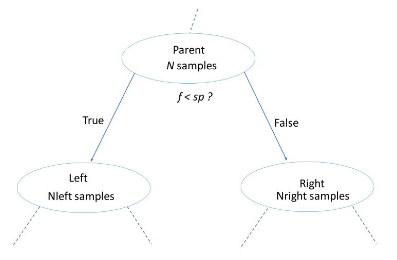
Information Gain (IG)

information gain $$ IG(\underbrace{f}_{\text{feature}}, \underbrace{sp}_{\text{split-point}} ) = I(\text{parent}) - \big( \frac{N_{\text{left}}}{N}I(\text{left}) + \frac{N_{\text{right}}}{N}I(\text{right}) \big) $$ - Criteria to measure the impurity of a note $I(\text{node})$: - gini index - entropy - etc...

Classification-Tree Learning
- Nodes are grown recursively.
- At each node, split the data based on:
  - feature $f$ and split-point $sp$ to maximize $IG(\text{node})$.
  - If $IG(\text{node}) = 0$, declare the node a leaf

Using entropy as a criterion¶

In this exercise, you'll train a classification tree on the Wisconsin Breast Cancer dataset using entropy as an information criterion. You'll do so using all the 30 features in the dataset, which is split into 80% train and 20% test.

In [10]:

from sklearn.tree import DecisionTreeClassifier

# Instantiate dt_entropy, set 'entropy' as the information criterion
dt_entropy = DecisionTreeClassifier(max_depth=8, criterion='entropy', random_state=1)

# Fit dt_entropy to the training set
dt_entropy.fit(X_train, y_train)

Out[10]:

DecisionTreeClassifier(ccp_alpha=0.0, class_weight=None, criterion='entropy',
                       max_depth=8, max_features=None, max_leaf_nodes=None,
                       min_impurity_decrease=0.0, min_impurity_split=None,
                       min_samples_leaf=1, min_samples_split=2,
                       min_weight_fraction_leaf=0.0, presort='deprecated',
                       random_state=1, splitter='best')

Entropy vs Gini index¶

In this exercise you'll compare the test set accuracy of dt_entropy to the accuracy of another tree named dt_gini. The tree dt_gini was trained on the same dataset using the same parameters except for the information criterion which was set to the gini index using the keyword 'gini'.

In [11]:

dt_gini = DecisionTreeClassifier(max_depth=8, criterion='gini', random_state=1)
dt_gini.fit(X_train, y_train)

Out[11]:

DecisionTreeClassifier(ccp_alpha=0.0, class_weight=None, criterion='gini',
                       max_depth=8, max_features=None, max_leaf_nodes=None,
                       min_impurity_decrease=0.0, min_impurity_split=None,
                       min_samples_leaf=1, min_samples_split=2,
                       min_weight_fraction_leaf=0.0, presort='deprecated',
                       random_state=1, splitter='best')

In [12]:

from sklearn.metrics import accuracy_score

# Use dt_entropy to predict test set labels
y_pred = dt_entropy.predict(X_test)
y_pred_gini = dt_gini.predict(X_test)

# Evaluate accuracy_entropy
accuracy_entropy = accuracy_score(y_test, y_pred)
accuracy_gini = accuracy_score(y_test, y_pred_gini)

# Print accuracy_entropy
print("Accuracy achieved by using entropy: ", accuracy_entropy)

# Print accuracy_gini
print("Accuracy achieved by using gini: ", accuracy_gini)

Accuracy achieved by using entropy:  0.8947368421052632
Accuracy achieved by using gini:  0.8859649122807017

Decision tree for regression¶

Information Criterion for Regression Tree

$$ I(\text{node}) = \underbrace{\text{MSE}(\text{node})}_{\text{mean-squared-error}} = \dfrac{1}{N_{\text{node}}} \sum_{i \in \text{node}} \big(y^{(i)} - \hat{y}_{\text{node}} \big)^2 $$$$ \underbrace{\hat{y}_{\text{node}}}_{\text{mean-target-value}} = \dfrac{1}{N_{\text{node}}} \sum_{i \in \text{node}}y^{(i)}$$

Prediction

$$ \hat{y}_{\text{pred}}(\text{leaf}) = \dfrac{1}{N_{\text{leaf}}} \sum_{i \in \text{leaf}} y^{(i)}$$

Train your first regression tree¶

In this exercise, you'll train a regression tree to predict the mpg (miles per gallon) consumption of cars in the auto-mpg dataset using all the six available features.

Preprocess¶

In [13]:

mpg = pd.read_csv('./dataset/auto.csv')
mpg.head()

Out[13]:

	mpg	displ	hp	weight	accel	origin	size
0	18.0	250.0	88	3139	14.5	US	15.0
1	9.0	304.0	193	4732	18.5	US	20.0
2	36.1	91.0	60	1800	16.4	Asia	10.0
3	18.5	250.0	98	3525	19.0	US	15.0
4	34.3	97.0	78	2188	15.8	Europe	10.0

In [14]:

mpg = pd.get_dummies(mpg)

In [15]:

mpg.head()

Out[15]:

	mpg	displ	hp	weight	accel	size	origin_Asia	origin_Europe	origin_US
0	18.0	250.0	88	3139	14.5	15.0	0	0	1
1	9.0	304.0	193	4732	18.5	20.0	0	0	1
2	36.1	91.0	60	1800	16.4	10.0	1	0	0
3	18.5	250.0	98	3525	19.0	15.0	0	0	1
4	34.3	97.0	78	2188	15.8	10.0	0	1	0

In [16]:

X = mpg.drop('mpg', axis='columns')
y = mpg['mpg']

In [17]:

X_train, X_test, y_train, y_test = train_test_split(X, y, test_size=0.2, random_state=3)

In [18]:

from sklearn.tree import DecisionTreeRegressor

# Instantiate dt
dt = DecisionTreeRegressor(max_depth=8, min_samples_leaf=0.13, random_state=3)

# Fit dt to the training set
dt.fit(X_train, y_train)

Out[18]:

DecisionTreeRegressor(ccp_alpha=0.0, criterion='mse', max_depth=8,
                      max_features=None, max_leaf_nodes=None,
                      min_impurity_decrease=0.0, min_impurity_split=None,
                      min_samples_leaf=0.13, min_samples_split=2,
                      min_weight_fraction_leaf=0.0, presort='deprecated',
                      random_state=3, splitter='best')

Evaluate the regression tree¶

In this exercise, you will evaluate the test set performance of dt using the Root Mean Squared Error (RMSE) metric. The RMSE of a model measures, on average, how much the model's predictions differ from the actual labels. The RMSE of a model can be obtained by computing the square root of the model's Mean Squared Error (MSE).

In [19]:

from sklearn.metrics import mean_squared_error

# Compute y_pred
y_pred = dt.predict(X_test)

# Compute mse_dt
mse_dt = mean_squared_error(y_test, y_pred)

# Compute rmse_dt
rmse_dt = mse_dt ** (1/2)

# Print rmse_dt
print("Test set RMSE of dt: {:.2f}".format(rmse_dt))

Test set RMSE of dt: 4.37

Linear regression vs regression tree¶

In this exercise, you'll compare the test set RMSE of dt to that achieved by a linear regression model. We have already instantiated a linear regression model lr and trained it on the same dataset as dt.

Preprocess¶

In [20]:

from sklearn.linear_model import LinearRegression

lr = LinearRegression()

lr.fit(X_train, y_train)

Out[20]:

LinearRegression(copy_X=True, fit_intercept=True, n_jobs=None, normalize=False)

In [21]:

# Predict test set labels
y_pred_lr = lr.predict(X_test)

# Compute mse_lr
mse_lr = mean_squared_error(y_test, y_pred_lr)

# Compute rmse_lr
rmse_lr = mse_lr ** 0.5

# Print rmse_lr
print("Linear Regression test set RMSE: {:.2f}".format(rmse_lr))

# Print rmse_dt
print("Regression Tree test set RMSE: {:.2f}".format(rmse_dt))

Linear Regression test set RMSE: 5.10
Regression Tree test set RMSE: 4.37