Riskfolio-Lib Tutorial:¶

__[Financionerioncios](https://financioneroncios.wordpress.com)__
__[Orenji](https://www.linkedin.com/company/orenj-i)__
__[Riskfolio-Lib](https://riskfolio-lib.readthedocs.io/en/latest/)__
__[Dany Cajas](https://www.linkedin.com/in/dany-cajas/)__

Tutorial 13: Riskfolio-Lib and Xlwings¶

1. Downloading the data:¶

In [1]:

import numpy as np
import pandas as pd
import yfinance as yf
import warnings

warnings.filterwarnings("ignore")
pd.options.display.float_format = '{:.4%}'.format

# Date range
start = '2016-01-01'
end = '2019-12-30'

# Tickers of assets
assets = ['JCI', 'TGT', 'CMCSA', 'CPB', 'MO', 'APA', 'MMC', 'JPM',
          'ZION', 'PSA', 'BAX', 'BMY', 'LUV', 'PCAR', 'TXT', 'TMO',
          'DE', 'MSFT', 'HPQ', 'SEE', 'VZ', 'CNP', 'NI', 'T', 'BA']
assets.sort()

# Downloading data
data = yf.download(assets, start = start, end = end)
data = data.loc[:,('Adj Close', slice(None))]
data.columns = assets

[*********************100%***********************]  25 of 25 completed

In [2]:

# Calculating returns

Y = data[assets].pct_change().dropna()

display(Y.head())

	APA	BA	BAX	BMY	CMCSA	CNP	CPB	DE	HPQ	JCI	...	NI	PCAR	PSA	SEE	T	TGT	TMO	TXT	VZ	ZION
Date
2016-01-05	-2.0257%	0.4057%	0.4035%	1.9693%	0.0180%	0.9305%	0.3678%	0.5783%	0.9483%	-1.1954%	...	1.5881%	0.0212%	2.8236%	0.9758%	0.6987%	1.7539%	-0.1730%	0.2410%	1.3734%	-1.0857%
2016-01-06	-11.4863%	-1.5879%	0.2412%	-1.7557%	-0.7727%	-1.2473%	-0.1736%	-1.1239%	-3.5867%	-0.9551%	...	0.5547%	0.0212%	0.1592%	-1.5646%	-0.1466%	-1.0155%	-0.7653%	-3.0048%	-0.9034%	-2.9145%
2016-01-07	-5.1389%	-4.1922%	-1.6573%	-2.7699%	-1.1047%	-1.9769%	-1.2207%	-0.8855%	-4.6059%	-2.5394%	...	-2.2066%	-3.0309%	-1.0410%	-3.1557%	-1.6148%	-0.2700%	-2.2845%	-2.0570%	-0.5492%	-3.0019%
2016-01-08	0.2737%	-2.2705%	-1.6037%	-2.5425%	0.1099%	-0.2241%	0.5707%	-1.6402%	-1.7641%	-0.1649%	...	-0.1538%	-1.1366%	-0.7308%	-0.1448%	0.0895%	-3.3839%	-0.1117%	-1.1386%	-0.9719%	-1.1254%
2016-01-11	-4.3384%	0.1693%	-1.6851%	-1.0215%	0.0915%	-1.1791%	0.5674%	0.5287%	0.6616%	0.0330%	...	1.6435%	0.0000%	0.9869%	-0.1450%	1.2224%	1.4570%	0.5367%	-0.4607%	0.5800%	-1.9918%

5 rows × 25 columns

2. Estimating Mean Variance Portfolios¶

2.1 Calculating the portfolio that maximizes Sharpe ratio.¶

In [3]:

import riskfolio as rp

# Building the portfolio object
port = rp.Portfolio(returns=Y)

# Calculating optimal portfolio

# Select method and estimate input parameters:

method_mu='hist' # Method to estimate expected returns based on historical data.
method_cov='hist' # Method to estimate covariance matrix based on historical data.

port.assets_stats(method_mu=method_mu, method_cov=method_cov)

# Estimate optimal portfolio:

model='Classic' # Could be Classic (historical), BL (Black Litterman) or FM (Factor Model)
rm = 'MV' # Risk measure used, this time will be variance
obj = 'Sharpe' # Objective function, could be MinRisk, MaxRet, Utility or Sharpe
hist = True # Use historical scenarios for risk measures that depend on scenarios
rf = 0 # Risk free rate
l = 0 # Risk aversion factor, only useful when obj is 'Utility'

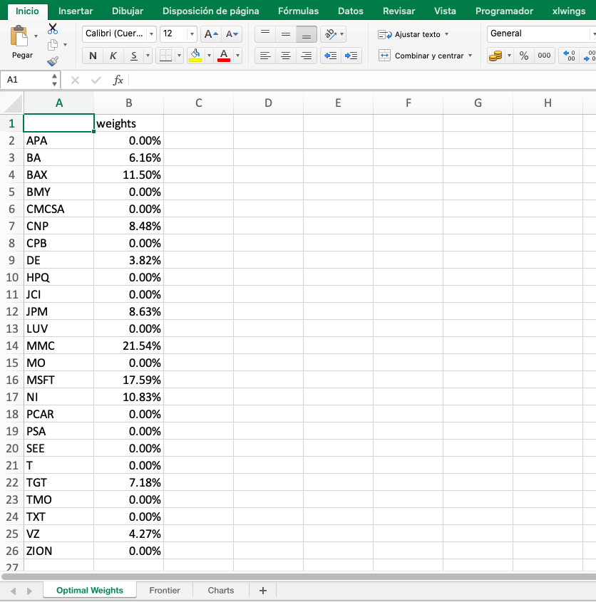
w = port.optimization(model=model, rm=rm, obj=obj, rf=rf, l=l, hist=hist)

display(w.T)

	APA	BA	BAX	BMY	CMCSA	CNP	CPB	DE	HPQ	JCI	...	NI	PCAR	PSA	SEE	T	TGT	TMO	TXT	VZ	ZION
weights	0.0000%	6.1590%	11.5019%	0.0000%	0.0000%	8.4807%	0.0000%	3.8193%	0.0000%	0.0000%	...	10.8262%	0.0000%	0.0000%	0.0000%	0.0000%	7.1805%	0.0000%	0.0000%	4.2738%	0.0000%

1 rows × 25 columns

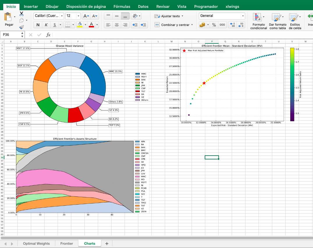
2.2 Plotting portfolio composition¶

In [4]:

import matplotlib.pyplot as plt

# Plotting the composition of the portfolio

fig_1, ax_1 = plt.subplots(figsize=(10,6))

ax_1 = rp.plot_pie(w=w, title='Sharpe Mean Variance', others=0.05, nrow=25, cmap = "tab20",
                   height=6, width=10, ax=ax_1)

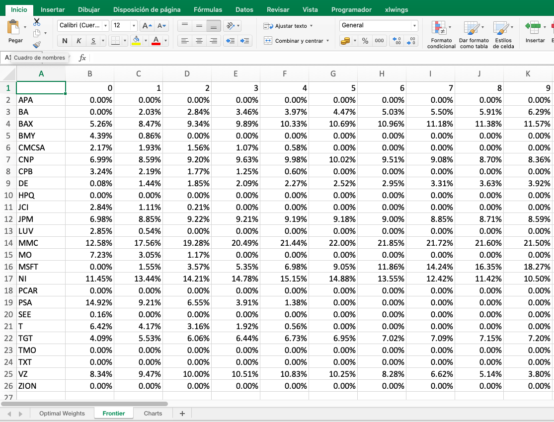
2.3 Calculate efficient frontier¶

In [5]:

points = 50 # Number of points of the frontier

frontier = port.efficient_frontier(model=model, rm=rm, points=points, rf=rf, hist=hist)

display(frontier.T.head())

	APA	BA	BAX	BMY	CMCSA	CNP	CPB	DE	HPQ	JCI	...	NI	PCAR	PSA	SEE	T	TGT	TMO	TXT	VZ	ZION
0	0.0000%	0.0000%	5.2634%	4.3887%	2.1705%	6.9871%	3.2390%	0.0790%	0.0000%	2.8377%	...	11.4508%	0.0000%	14.9184%	0.1628%	6.4196%	4.0904%	0.0000%	0.0000%	8.3446%	0.0001%
1	0.0000%	2.0325%	8.4718%	0.8579%	1.9327%	8.5940%	2.1945%	1.4376%	0.0000%	1.1060%	...	13.4410%	0.0000%	9.2132%	0.0000%	4.1682%	5.5285%	0.0000%	0.0000%	9.4731%	0.0000%
2	0.0000%	2.8407%	9.3407%	0.0000%	1.5588%	9.1990%	1.7699%	1.8516%	0.0000%	0.2108%	...	14.2140%	0.0000%	6.5518%	0.0000%	3.1594%	6.0608%	0.0000%	0.0000%	9.9971%	0.0000%
3	0.0000%	3.4597%	9.8935%	0.0000%	1.0711%	9.6311%	1.2504%	2.0914%	0.0000%	0.0000%	...	14.7829%	0.0000%	3.9064%	0.0000%	1.9201%	6.4433%	0.0000%	0.0000%	10.5067%	0.0000%
4	0.0000%	3.9674%	10.3314%	0.0000%	0.5839%	9.9784%	0.6012%	2.2744%	0.0000%	0.0000%	...	15.1468%	0.0000%	1.3826%	0.0000%	0.5558%	6.7335%	0.0000%	0.0000%	10.8300%	0.0000%

5 rows × 25 columns

In [6]:

# Plotting the efficient frontier

label = 'Max Risk Adjusted Return Portfolio' # Title of point
mu = port.mu # Expected returns
cov = port.cov # Covariance matrix
returns = port.returns # Returns of the assets

fig_2, ax_2 = plt.subplots(figsize=(10,6))

rp.plot_frontier(w_frontier=frontier, mu=mu, cov=cov, returns=returns, rm=rm,
                 rf=rf, alpha=0.01, cmap='viridis', w=w, label=label,
                 marker='*', s=16, c='r', height=6, width=10, ax=ax_2)

Out[6]:

<AxesSubplot:title={'center':'Efficient Frontier Mean - Standard Deviation (MV)'}, xlabel='Expected Risk - Standard Deviation (MV)', ylabel='Expected Return'>

In [7]:

# Plotting efficient frontier composition

fig_3, ax_3 = plt.subplots(figsize=(10,6))

rp.plot_frontier_area(w_frontier=frontier, cmap="tab20", height=6, width=10, ax=ax_3)

Out[7]:

<AxesSubplot:title={'center':"Efficient Frontier's Assets Structure"}>

3. Combining Riskfolio-Lib and Xlwings¶

3.1 Creating an Empty Excel Workbook¶

In [8]:

import xlwings as xw

# Creating an empty Excel Workbook

wb = xw.Book()  
sheet1 = wb.sheets[0]
sheet1.name = 'Charts'
sheet2 = wb.sheets.add('Frontier')
sheet3 = wb.sheets.add('Optimal Weights')

3.2 Adding Pictures to Sheet 1¶

In [9]:

sheet1.pictures.add(fig_1, name = "Weights",
                    update = True, 
                    top = sheet1.range("A1").top,
                    left = sheet1.range("A1").left)

sheet1.pictures.add(fig_2, name = "Frontier",
                    update = True, 
                    top = sheet1.range("M1").top,
                    left = sheet1.range("M1").left)

sheet1.pictures.add(fig_3, name = "Composition",
                    update = True, 
                    top = sheet1.range("A30").top,
                    left = sheet1.range("A30").left)

Out[9]:

<Picture 'Composition' in <Sheet [Libro2]Charts>>

3.2 Adding Data to Sheet 2 and Sheet 3¶

In [10]:

# Writing the weights of the frontier in the Excel Workbook

sheet2.range('A1').value = frontier.applymap('{:.6%}'.format)

# Writing the optimal weights in the Excel Workbook

sheet3.range('A1').value = w.applymap('{:.6%}'.format)