%load_ext load_style
%load_style talk.css
Overview of the IPython notebook
from IPython.display import display, HTML
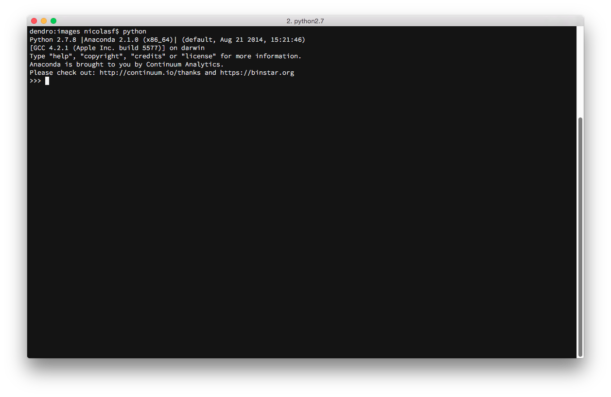
Python ships with a basic interactive interpreter ... not much fun here

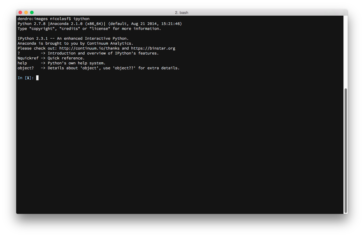
IPython is an enhanced interactive interpreter, developped for scientific development, adding e.g. history, tab-completion, interactive help, and lots and lots of goodies:

Since 2005, the IPython development team has introduced the IPython notebook. This is a web application, running in the browser, that is connected to a Python kernel running in the background.
HTML('<iframe src=http://ipython.org/notebook.html width=900 height=350></iframe>')
It behaves as an interactive notebook, in which you can weave Python code and outputs, figures generated from Python / matplotlib, images (either local and remote), websites, videos and richly formatted comments using markdown, which is a superset of HTML with a very simple syntax (see here for more)
It is structured into executable cells, into which by default you can run arbitrary python code
It has a sophisticated tab completion and help system
The power of IPython comes in part because of its numerous extensions and magic functions
And finally you can export a notebook in different formats, including HTML and Latex (and PDF).
Recently the IPython notebook as been featured in the toolbox section of Nature
HTML('<iframe src=http://www.nature.com/news/interactive-notebooks-sharing-the-code-1.16261 width=1000 height=350></iframe>')
Using the IPython notebook
### This is a code cell, containing python code, it is executed by <shift>-<enter> or <alt>-<enter>

def func(x):
    return x**3

[func(x) for x in xrange(10)]
Getting help
%quickref
IPython has a sophisticated help and tab completion system, which allows introspection: i.e.
If you want details regarding the properties and functionality of any Python objects currently loaded into IPython, you can use the ? to reveal any details that are available:
some_dict = {}
some_dict?
from numpy import random
random?
help(random) # produces a long output below instead of in a dedicated frame. <CTRL>-<M> <D>
Tab completion
Because IPython allows for introspection, it is able to afford the user the ability to tab-complete commands that have been partially typed. This is done by pressing the <tab> key at any point during the process of typing a command:
listA = [1, 2., 'sentence', 1, (1,2), {'answer': 42}] # here I construct a LIST containing different items
listA.
listA.count(1)
listA.count(2.0)
And opening a parenthesis and pressing <tab> gives details about the arguments of a function or method
listA.count()
listA
including markdown comments
A short introduction to markdown syntax
Using markdown cells, you can insert formatted comments, observations ... directly in between executable code and outputs ...
To toggle from code cell (the default) to markdown cell, you can use the toolbar, or <ctrl>-<m> + <m> (<command>-<m> + <m> on Macs)
You can italicize, boldface
build
lists
enumerate
stuff
and embed syntax highlighted code meant for illustration instead of execution in Python:
def f(x):
    """a docstring"""
    return x**2
or other languages:
if (i=0; i<n; i++) {
  printf("hello %d\n", i);
  x += 4;
}
You can insert images seemlessly into a Markdown cell, but if it is local instead of on the web, it needs to reside in an images folder in the same directory as your notebook.
The syntax is then

e.g.

Thanks to MathJax, you can include mathematical expressions in a markdown cell using Latex syntax both inline and displayed:
For example $e^{i\pi} + 1 = 0$ becomes $e^{i\pi} + 1 = 0$
and
$$e^x=\sum_{i=0}^\infty \frac{1}{i!}x^i$$
becomes:
$$e^x=\sum_{i=0}^\infty \frac{1}{i!}x^i$$
Mathjax is a JavaScript library, and by default IPython uses the online version, if you want to be able to use it offline, you need to install MathJax locally by running that (once) in a code cell:
from IPython.external.mathjax import install_mathjax
install_mathjax()
The IPython notebook rich display system
from IPython.display import Image, YouTubeVideo
### that will display a frame with specified width and height ...

HTML('<iframe src="http://numpy.org/" height=300 width=600>'
     '</iframe>')
### This inserts an image in the output cell

Image(filename='images/lost_wormhole.jpg',width=500)
### This embeds a video from YouTube
### You can embed Vimeo videos by calling from IPython.display import VimeoVideo

# Fernando Pérez at PyConCA, here I start at 30 minutes
YouTubeVideo('F4rFuIb1Ie4', start = 30*60)
### You can also embed a LOCAL video in the notebook, but have to encode it: Not sure it will work
### on Windows ...

import io
import base64

filename = './data/Astro_ML_PYDATA2012.mp4'

video = io.open(filename, 'r+b').read()
encoded = base64.b64encode(video)
HTML(data='''<video alt="AstroML talk" controls>
           <source src="data:video/mp4;base64,{0}" type="video/mp4" />
           </video>'''.format(encoded.decode('ascii')))
Inline plots with matplotlib
import numpy as np
import matplotlib.pyplot as plt
# this is a magic IPython command (%) allowing matplotlib plots to be displayed inline in the notebook
%matplotlib inline
t = np.linspace(0, 2*np.pi, 100)
plt.plot(np.sin(t))
# you can also choose to display figure OUTSIDE the notebook
# the available backends are [inline|qt|osx|gtx] ... For Windows try qt
%matplotlib osx
t = np.linspace(0, 2*np.pi, 100)
plt.plot(np.sin(t))
from version 1.4 of Matplotlib, a special interactive backend for the IPython notebook is available
You need to restart the kernel and then run the following cell for it to work
import matplotlib
matplotlib.use('nbagg')
%matplotlib inline
Some useful magic commands in IPython
# for a list of available magic command

%lsmagic
For example
%whos
list all variables (incl. classes, functions, etc) in the namespace
%whos
Writing the content of a cell to file
%%file tmp.py
#!/usr/bin/env python
import numpy as np

print('Hello world')

a = np.arange(10) ### will be available in the namespace
Running some external python script (local or online)
%run tmp.py
a
Loading the content of some local python script (you can load actually anything, e.g. a Markdown file)
%load tmp.py
#!/usr/bin/env python
import numpy as np

print('Hello world')

a = np.arange(10) ### will be available in the namespace
works as well for scripts available online
### loading an example from the matplotlib gallery

%load http://matplotlib.org/mpl_examples/images_contours_and_fields/streamplot_demo_features.py
"""
Demo of the `streamplot` function.

A streamplot, or streamline plot, is used to display 2D vector fields. This
example shows a few features of the stream plot function:

    * Varying the color along a streamline.
    * Varying the density of streamlines.
    * Varying the line width along a stream line.
"""
import numpy as np
import matplotlib.pyplot as plt

Y, X = np.mgrid[-3:3:100j, -3:3:100j]
U = -1 - X**2 + Y
V = 1 + X - Y**2
speed = np.sqrt(U*U + V*V)

plt.streamplot(X, Y, U, V, color=U, linewidth=2, cmap=plt.cm.autumn)
plt.colorbar()

f, (ax1, ax2) = plt.subplots(ncols=2)
ax1.streamplot(X, Y, U, V, density=[0.5, 1])

lw = 5*speed/speed.max()
ax2.streamplot(X, Y, U, V, density=0.6, color='k', linewidth=lw)

plt.show()
Interacting with the OS: the IPython notebook as an enhanced shell
!rm tmp.py ### ! escapes to the OS (!del tmp.py on windows)
notebooks = !ls *.ipynb ### notebooks is a python list ... not sure how to use wildcards on Windows
notebooks
And if you need to actually quickly put together and run a bash script (linux / Mac), you don't need to escape the IPython notebook thanks to the
%%bash
cell magic ...
%%bash

# Substitutes underscores for blanks in all the filenames in a directory.

ONE=1                     # For getting singular/plural right (see below).
number=0                  # Keeps track of how many files actually renamed.
FOUND=0                   # Successful return value.

for filename in *         # Traverses all files in directory.
do
     echo "$filename" | grep -q " "         # Checks whether filename
     if [ $? -eq $FOUND ]                   # contains space(s).
     then
       fname=$filename                      # Strips off path.
       n=`echo $fname | sed -e "s/ /_/g"`   # Substitutes underscore for blank.
       mv "$fname" "$n"                     # Do the actual renaming.
       let "number += 1"
     fi
done

if [ "$number" -eq "$ONE" ]                 # For correct grammar.
then
 echo "$number file renamed."
else
 echo "$number files renamed."
fi

exit 0
Exporting your notebook in other formats
A notebook (extension .ipynb) is actually just a JSON file, using built-in converters (with the help of pandoc) you can convert a notebook into a variety of formats for sharing, illustration, publishing, etc.
#!ipython nbconvert --help
!ipython nbconvert --help
name = 'IPython_notebook'
!ipython nbconvert {name}.ipynb --to html
display(HTML("<a href='{name}.html' target='_blank'> {name}.html </a>".format(name=name)))
!open ./{name}.html
Sharing your IPython notebook
- host your IPython notebook on the public internet (e.g. github repo, github gist)
- go to http://nbviewer.ipython.org/ and copy the URL
- Et voila !