< Modules | Convolutional Neural Networks | Transfer Learning >¶

Convolutional Neural Networks¶

In this notebook, we first give a short introduction to convolutions, which are a prerequisite to understand how CNNs work.
Then, we will write code to create a CNN, load the data and train our model.

Table of Contents¶

1. What is a convolution ?¶

2. Building a CNN ¶

3. Training our CNN ¶

In [ ]:

! pip -q install colorama
! wget -q https://github.com/theevann/amld-pytorch-workshop/raw/master/figures/image-city.jpg

In [ ]:

import sys
import colorama
from collections import OrderedDict
from matplotlib import pyplot as plt 

import torch
import torch.nn as nn
import torch.nn.functional as F
import torch.optim as optim

torch.set_printoptions(precision=3)

What is a convolution ?¶

Note: Below are intuitive and practical explanations that do not intent to be mathematically rigorous. This is intentional to make the understanding easier.

1D Convolution¶

A convolution is an operation between two signals.
In computer vision, one signal is usually the input (audio signal, image, ...), while the other signal is called filter or kernel.

To get the convolution output of an input vector and a kernel:

Slide the kernel at each different possible positions in the input
For each position, perform the element-wise product between the kernel and the corresponding part of the input
Sum the result of the element-wise product

convolution 1d

We can perform this operation in PyTorch using the conv_1d function.

In [ ]:

input = torch.Tensor([1,4,-1,0,2,-2,1,3,3,1]).view(1,1,-1)  # Size: (Batch size, Num Channels, Input size)
kernel = torch.Tensor([1,2,0,-1]).view(1,1,-1)  # Size: (Num output channels, Num input channels, Kernel size)

torch.nn.functional.conv1d(input, kernel)

2D Convolution¶

The extension to 2D is straightforward: the operation is similar, but now input and kernel are both 2-dimensional.

convolution 2d

We can perform this operation in PyTorch using the conv_2d function.

In [ ]:

# Input Size: (Batch size, Num channels, Input height, Input width)
input = torch.Tensor([[3,3,2,1,0], [0,0,1,3,1], [3,1,2,2,3], [2,0,0,2,2], [2,0,0,0,1]]).view(1,1,5,5)

# Kernel Size: (Num output channels, Num input channels, Kernel height, Kernel width)
kernel = torch.Tensor([[0,1,2],[2,2,0],[0,1,2]]).view(1,1,3,3)

torch.nn.functional.conv2d(input, kernel)

Multiple channels¶

You can use have multiple channels in input. A color image usually have 3 input channels : RGB.
Therefore, the kernel will also have channels, one for each input channel.

You can use multiple different kernels. The number of output channels corresponds to the number of kernel you use.

Trying on a real image¶

In [ ]:

from PIL import Image

image = Image.open("image-city.jpg")
print(image.size)
image

Your Turn !¶

Fill in the code cell below to perform the convolution of the above image with a kernel.
We will use a boundary detector filter as kernel:

$$\begin{bmatrix} -1 & 0 & 1 \\ -1 & 0 & 1 \\ -1 & 0 & 1 \end{bmatrix} $$

Pay attention to the dimensions of the input and the kernel:

Input Size: Batch size x Num channels x Input height x Input width
Kernel Size: Num output channels x Num input channels x Kernel height x Kernel width

Note:

There are 3 input channels (since we have an rgb image)
In output, we want only one channel (ie. we define only one kernel)
Here, batch size will be 1.

In [ ]:

# %load -r 1-8 solutions/solution_5.py
from torchvision.transforms.functional import to_tensor, to_pil_image

image_tensor = to_tensor(image)
input = image_tensor.unsqueeze(0)
kernel = torch.Tensor([-1,0,1]).expand(1,3,3,3)

out =  torch.nn.functional.conv2d(input, kernel)

In [ ]:

norm_out = (out - out.min()) / (out.max() - out.min())  # Map output to [0,1] for visualisation purposes
to_pil_image(norm_out.squeeze())

Convolutions in `nn.Module`¶

When using a convolution layer inside an nn.Module, we rather use the nn.Conv2d module.
The kernels of the convolution are directly instantiated by nn.Conv2d.

In [ ]:

conv_1 = nn.Conv2d(in_channels=3, out_channels=2, kernel_size=(3,3))

print("Convolution", conv_1)
print("Kernel size: ", conv_1.weight.shape) # First two dimensions are: Num output channels and Num input channels

In [ ]:

# Fake 5x5 input with 3 channels
input = torch.randn(1, 3, 5, 5)  # batch_size, num_channels, height, width

out = conv_1(input)
print(out)

Animations credits: Francois Fleuret, Vincent Dumoulin

Building a CNN¶

We will use the MNIST classification dataset again as our learning task. However, this time we will try to solve it using Convolutional Neural Networks. Let's build the LeNet-5 CNN with PyTorch !

Defining the LeNet-5 architecture¶

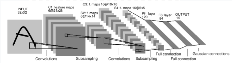
Y. LeCun, L. Bottou, Y. Bengio, and P. Haffner. "Gradient-based learning applied to document recognition." Proceedings of the IEEE, 86(11):2278-2324, November 1998.

Note: The Gaussian connections in the last layer were used to estimate the lack of fit. In our implementation, we use a cross-entropy loss function as it's common nowadays. Similarly, ReLU are used instead of tanh activation.

Architecture Details

Convolutional part:

Layer	Name	Input channels	Output channels	Kernel	stride
Convolution	C1	1	6	5x5	1
ReLU		6	6
MaxPooling	S2	6	6	2x2	2
Convolution	C3	6	16	5x5	1
ReLU		16	16
MaxPooling	S4	16	16	2x2	2
Convolution	C5	16	120	5x5	1
ReLU		120	120

Fully Connected part:

Layer	Name	Input size	Output size
Linear	F5	120	84
ReLU
Linear	F6	84	10
LogSoftmax

Your turn !¶

Write a Pytorch module for the LeNet-5 model.
You may need to use : nn.Sequential, nn.Conv2d, nn.ReLU, nn.MaxPool2d, nn.Linear, nn.LogSoftmax, nn.Flatten

In [ ]:

# %load -s LeNet5 solutions/solution_5.py

class LeNet5(nn.Module):
    def __init__(self):
        super(LeNet5, self).__init__()

        # YOUR TURN
        
    def forward(self, imgs):
        
        # YOUR TURN
        
        return output

An extensive list of all available layer types can be found on https://pytorch.org/docs/stable/nn.html.

Print a network summary¶

In [ ]:

conv_net = LeNet5()
print(conv_net)

Retrieve trainable parameters¶

In [ ]:

named_params = list(conv_net.named_parameters())
print("len(params): %s\n" % len(named_params))

for name, param in named_params:
    print("%s:\t%s" % (name, param.shape))

Feed network with a random input¶

In [ ]:

input = torch.randn(1, 1, 32, 32)  # batch_size, num_channels, height, width
out = conv_net(input)
print("Log-Probabilities: \n%s\n" % out)
print("Probabilities: \n%s\n" % torch.exp(out))
print("out.shape: \n%s" % (out.shape,))

Training our CNN¶

Train function¶

Similarly to the previous notebook, we define a train function train_cnn.

In [ ]:

def train_cnn(model, train_loader, test_loader, device, num_epochs=3, lr=0.1):

    # define an optimizer and a loss function
    optimizer = torch.optim.Adam(model.parameters(), lr=lr)
    criterion = torch.nn.CrossEntropyLoss()

    for epoch in range(num_epochs):
        print("=" * 40, "Starting epoch %d" % (epoch + 1), "=" * 40)
        
        model.train()  # Not necessary in our example, but still good practice.
                       # Only models with nn.Dropout and nn.BatchNorm modules require it
                
        # dataloader returns batches of images for 'data' and a tensor with their respective labels in 'labels'
        for batch_idx, (data, labels) in enumerate(train_loader):
            data, labels = data.to(device), labels.to(device)

            optimizer.zero_grad()
            output = model(data)
            loss = criterion(output, labels)
            loss.backward()
            optimizer.step()
            
            if batch_idx % 40 == 0:
                print("Batch %d/%d, Loss=%.4f" % (batch_idx, len(train_loader), loss.item()))
        
        # Compute the train and test accuracy at the end of each epoch
        train_acc = accuracy(model, train_loader, device)
        test_acc = accuracy(model, test_loader, device)
        
        print(colorama.Fore.GREEN, "\nAccuracy on training: %.2f%%" % (100*train_acc))
        print("Accuracy on test: %.2f%%" % (100*test_acc), colorama.Fore.RESET)

Test function¶

We also define an accuracy function which can evaluate our model's accuracy on train/test data

In [ ]:

def accuracy(model, dataloader, device):
    """ Computes the model's accuracy on the data provided by 'dataloader'
    """
    model.eval()
    
    num_correct = 0
    num_samples = 0
    with torch.no_grad():  # deactivates autograd, reduces memory usage and speeds up computations
        for data, labels in dataloader:
            data, labels = data.to(device), labels.to(device)

            predictions = model(data).max(1)[1]  # indices of the maxima along the second dimension
            num_correct += (predictions == labels).sum().item()
            num_samples += predictions.shape[0]
        
    return num_correct / num_samples

Loading the train and test data with `dataloaders`¶

In [ ]:

from torchvision import datasets, transforms

transformations = transforms.Compose([
    transforms.Resize((32, 32)),
    transforms.ToTensor()
])

train_data = datasets.MNIST('./data', 
                            train = True, 
                            download = True,
                            transform = transformations)

test_data = datasets.MNIST('./data', 
                            train = False, 
                            download = True,
                            transform = transformations)

train_loader = torch.utils.data.DataLoader(train_data, batch_size=256, shuffle=True)
test_loader = torch.utils.data.DataLoader(test_data, batch_size=1024, shuffle=False)

Start the training!¶

In [ ]:

device = torch.device('cuda' if torch.cuda.is_available() else 'cpu')
conv_net.to(device)

train_cnn(conv_net, train_loader, test_loader, device, lr=2e-3)

Let's look at some of the model's predictions¶

In [ ]:

def visualize_predictions(model, dataloader, device):
    data, labels = next(iter(dataloader))
    data, labels = data[:10].to(device), labels[:10]
    predictions = model(data).max(1)[1]
    
    predictions, data = predictions.cpu(), data.cpu()
    
    plt.figure(figsize=(16,9))
    for i in range(10):
        img = data.squeeze(1)[i]
        plt.subplot(1, 10, i+1)
        plt.imshow(img, cmap="gray", interpolation="none")
        plt.xlabel(predictions[i].item(), fontsize=18)
        plt.xticks([])
        plt.yticks([])    
    
visualize_predictions(conv_net, test_loader, device)

< Modules | Convolutional Neural Networks | Transfer Learning >¶

< Modules | Convolutional Neural Networks | Transfer Learning >¶

Convolutional Neural Networks¶

Table of Contents¶

1. What is a convolution ?¶

2. Building a CNN¶

3. Training our CNN¶

What is a convolution ?¶

1D Convolution¶

2D Convolution¶

Multiple channels¶

Trying on a real image¶

Your Turn !¶

Convolutions in nn.Module¶

Building a CNN¶

Defining the LeNet-5 architecture¶

Your turn !¶

Print a network summary¶

Retrieve trainable parameters¶

Feed network with a random input¶

Training our CNN¶

Train function¶

Test function¶

Loading the train and test data with dataloaders¶

Start the training!¶

Let's look at some of the model's predictions¶

< Modules | Convolutional Neural Networks | Transfer Learning >¶

2. Building a CNN ¶

3. Training our CNN ¶

Convolutions in `nn.Module`¶

Loading the train and test data with `dataloaders`¶